Chapter 5 Standardization and the normal distribution
5.1 Data standardization (z-score)
Sometimes tools of mathematical statistics, machine learning, or data analysis require the standardization of quantitative data. Standardizing a set of numbers involves transforming the data using the following formula:
\[ z = \frac{x - \text{mean}}{\text{standard deviation}} \tag{5.1} \]
This produces standardized values, or “z-scores.”
5.2 Normal distribution
The normal distribution is a mathematical tool useful for modeling many sets of quantitative data. The distribution of many natural and social phenomena is approximately normal — for example, human height, newborn weight, or other biological characteristics, deviations of temperature from the long-term average, or measurement errors. The distribution of the sample mean in repeated sampling also approaches the normal distribution as the sample size increases. For data that follow or approximate the normal distribution, the histogram takes on a characteristic bell shape (hence the term “bell curve”).
5.3 Empirical rule
For a normal or approximately normal distribution3:
about 68% of values lie within one standard deviation from the mean,
about 95% of values lie within two standard deviations from the mean,
about 99.7% of values (almost all) lie within three standard deviations from the mean.
The empirical rule works quite well for many datasets but not for all of them.
In particular, in many real datasets, the standard deviation can be roughly estimated based on the 95% rule. This is why the standard deviation is often interpreted through the lens of the empirical rule.
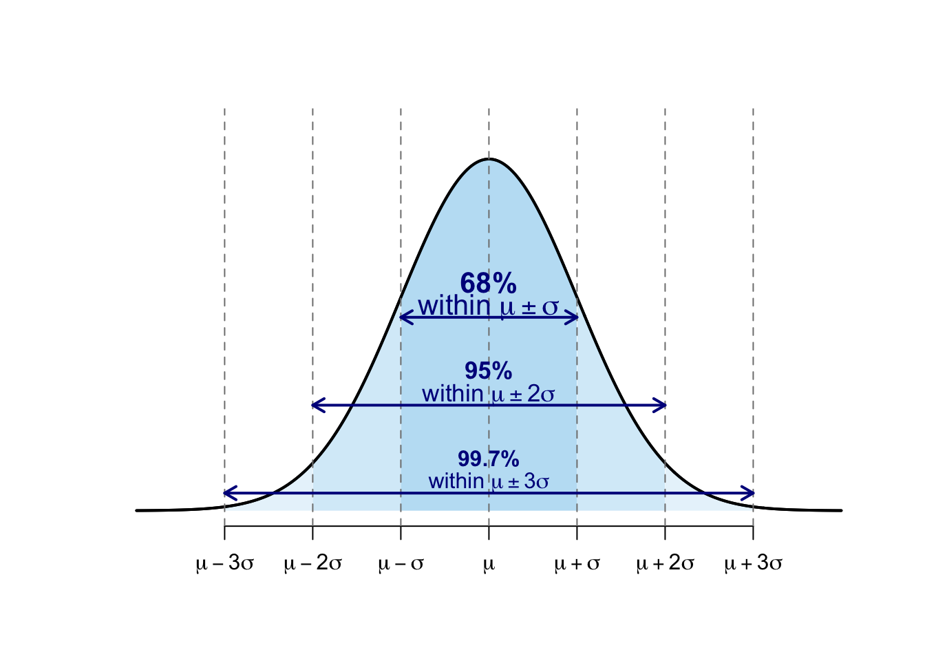
Figure 5.1: Empirical rule for normal distributions – illustration.
5.4 Chebyshev’s Inequality
The empirical rule works well for bell-shaped data, but not all datasets look like that. Chebyshev’s inequality is more general — it applies to any dataset, no matter its shape. According to Chebyshev’s rule:
at least 75% of values are within two standard deviations from the mean,
at least 89% within three,
at least 94% within four.
Chebyshev’s rule gives minimum values, not exact ones. It’s useful when data are skewed or irregular.
| Distance from the mean | Empirical rule (normal) | Chebyshev’s rule (any shape) |
|---|---|---|
| 1 SD | ~68% | — |
| 2 SD | ~95% | ≥75% |
| 3 SD | ~99.7% | ≥89% |
| 4 SD | ~100% | ≥94% |
5.5 Test questions
Question 5.1 The height in a certain group of men is approximately normally distributed with a mean of 179 and a standard deviation of 7.
Adam is 186 cm tall. His z-score is
Bruno is 172 cm tall. His z-score is
Conrad is 193 cm tall. His z-score is
Daniel is 179 cm tall. His z-score is
Emil is 161.5 cm tall. His z-score is
Question 5.2 The height in a certain group of men is approximately normally distributed with a mean of 179 and a standard deviation of 7.
What is the approximate probability that the height of a randomly selected man from this group will be between 172 cm and 186 cm?
What is the approximate probability that a randomly selected man from this group will be taller than 193 cm?
What is the approximate probability that a randomly selected man from this group will be shorter than 193 cm?
What is the approximate probability that a randomly selected man from this group will be taller than 172 cm?
Question 5.3 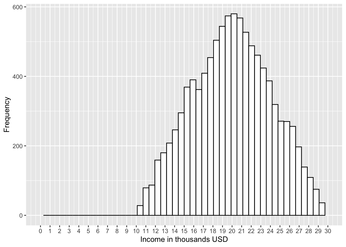
The histogram shows the distribution of incomes (in thousands of USD) in a certain population.
The average income in this population is approximately:
The first quartile in this population is approximately:
The standard deviation in this population is approximately:
For a normal distribution, these values, rounded to two decimal places, are: 68.27%, 95.45%, and 99.73%.↩︎