Chapter 6 Exploring Crime in Florida
My company has chosen me to investigate and uncover what socioeconomic factors are most strongly associated with rising crime rates across Florida counties. I’m super excited!
6.1 Loading and Preparing the Data
Now I’m going to load and clean the data.
library(readxl)
florida_crime <- read_excel("data/Florida County Crime Rates.xlsx")
head(florida_crime)
## # A tibble: 6 × 5
## County C I HS U
## <chr> <dbl> <dbl> <dbl> <dbl>
## 1 ALACHUA 104 22.1 82.7 73.2
## 2 BAKER 20 25.8 64.1 21.5
## 3 BAY 64 24.7 74.7 85
## 4 BRADFORD 50 24.6 65 23.2
## 5 BREVARD 64 30.5 82.3 91.9
## 6 BROWARD 94 30.6 76.8 98.96.1.1 Renaming columns and formatting county names
library(tidyverse)
florida_crime <- florida_crime %>%
  rename(
    Crime = "C",
    Income = "I",
    HighSchoolGrad = "HS",
    UrbanPop = "U"
  )
florida_crime
## # A tibble: 67 × 5
## County Crime Income HighSchoolGrad UrbanPop
## <chr> <dbl> <dbl> <dbl> <dbl>
## 1 ALACHUA 104 22.1 82.7 73.2
## 2 BAKER 20 25.8 64.1 21.5
## 3 BAY 64 24.7 74.7 85
## 4 BRADFORD 50 24.6 65 23.2
## 5 BREVARD 64 30.5 82.3 91.9
## 6 BROWARD 94 30.6 76.8 98.9
## 7 CALHOUN 8 18.6 55.9 0
## 8 CHARLOTTE 35 25.7 75.7 80.2
## 9 CITRUS 27 21.3 68.6 31
## 10 CLAY 41 34.9 81.2 65.8
## # ℹ 57 more rows##
## Attaching package: 'skimr'## The following object is masked from 'package:mosaic':
##
## n_missing## # A tibble: 67 × 5
## County Crime Income HighSchoolGrad UrbanPop
## <chr> <dbl> <dbl> <dbl> <dbl>
## 1 Alachua 104 22.1 82.7 73.2
## 2 Baker 20 25.8 64.1 21.5
## 3 Bay 64 24.7 74.7 85
## 4 Bradford 50 24.6 65 23.2
## 5 Brevard 64 30.5 82.3 91.9
## 6 Broward 94 30.6 76.8 98.9
## 7 Calhoun 8 18.6 55.9 0
## 8 Charlotte 35 25.7 75.7 80.2
## 9 Citrus 27 21.3 68.6 31
## 10 Clay 41 34.9 81.2 65.8
## # ℹ 57 more rows| Name | florida_crime |
| Number of rows | 67 |
| Number of columns | 5 |
| _______________________ | |
| Column type frequency: | |
| character | 1 |
| numeric | 4 |
| ________________________ | |
| Group variables | None |
Variable type: character
| skim_variable | n_missing | complete_rate | min | max | empty | n_unique | whitespace |
|---|---|---|---|---|---|---|---|
| County | 0 | 1 | 3 | 9 | 0 | 67 | 0 |
Variable type: numeric
| skim_variable | n_missing | complete_rate | mean | sd | p0 | p25 | p50 | p75 | p100 | hist |
|---|---|---|---|---|---|---|---|---|---|---|
| Crime | 0 | 1 | 52.40 | 28.19 | 0.0 | 35.50 | 52.0 | 69.00 | 128.0 | ▃▇▇▃▂ |
| Income | 0 | 1 | 24.51 | 4.68 | 15.4 | 21.05 | 24.6 | 28.15 | 35.6 | ▂▇▅▅▂ |
| HighSchoolGrad | 0 | 1 | 69.49 | 8.86 | 54.5 | 62.45 | 69.0 | 76.90 | 84.9 | ▇▇▆▇▆ |
| UrbanPop | 0 | 1 | 49.56 | 33.97 | 0.0 | 21.60 | 44.6 | 83.55 | 99.6 | ▅▆▂▃▇ |
##     County              Crime           Income      HighSchoolGrad
##  Length:67          Min.   :  0.0   Min.   :15.40   Min.   :54.50
##  Class :character   1st Qu.: 35.5   1st Qu.:21.05   1st Qu.:62.45
##  Mode  :character   Median : 52.0   Median :24.60   Median :69.00
##                     Mean   : 52.4   Mean   :24.51   Mean   :69.49
##                     3rd Qu.: 69.0   3rd Qu.:28.15   3rd Qu.:76.90
##                     Max.   :128.0   Max.   :35.60   Max.   :84.90
##     UrbanPop
##  Min.   : 0.00
##  1st Qu.:21.60
##  Median :44.60
##  Mean   :49.56
##  3rd Qu.:83.55
##  Max.   :99.60
6.2 Exploratory Data Analysis
Descriptive statistics for florida_crime.
##     County              Crime           Income      HighSchoolGrad
##  Length:67          Min.   :  0.0   Min.   :15.40   Min.   :54.50
##  Class :character   1st Qu.: 35.5   1st Qu.:21.05   1st Qu.:62.45
##  Mode  :character   Median : 52.0   Median :24.60   Median :69.00
##                     Mean   : 52.4   Mean   :24.51   Mean   :69.49
##                     3rd Qu.: 69.0   3rd Qu.:28.15   3rd Qu.:76.90
##                     Max.   :128.0   Max.   :35.60   Max.   :84.90
##     UrbanPop
##  Min.   : 0.00
##  1st Qu.:21.60
##  Median :44.60
##  Mean   :49.56
##  3rd Qu.:83.55
##  Max.   :99.60
By using the summary function (twice) we can take a look at the mean, median, and range of the dataset.
Mean Crime = 52.4, Mean Income = 24.15, Mean HighSchoolGrad = 69.49, Mean UrbanPop = 49.56 Median Crime = 52, Median Income = 24.60, Median HighSchoolGrad = 69, Median UrbanPop = 44.60 Range Crime = 0-128, Range Income = 15.40-35.60, Range HighSchoolGrad = 54.50-84.90, Range UrbanPop = 0-99.60
6.3 Visualizing the data in all its glory
viz1 <- ggplot(florida_crime, aes(x=Income, y=Crime))+
  geom_point(size=2.5)+
  geom_smooth(method = "lm", se=FALSE)+
  labs(
    title = "Income vs Crime",
    x = "Income",
    y = "Crime"
  )
print(viz1)
## `geom_smooth()` using formula = 'y ~ x'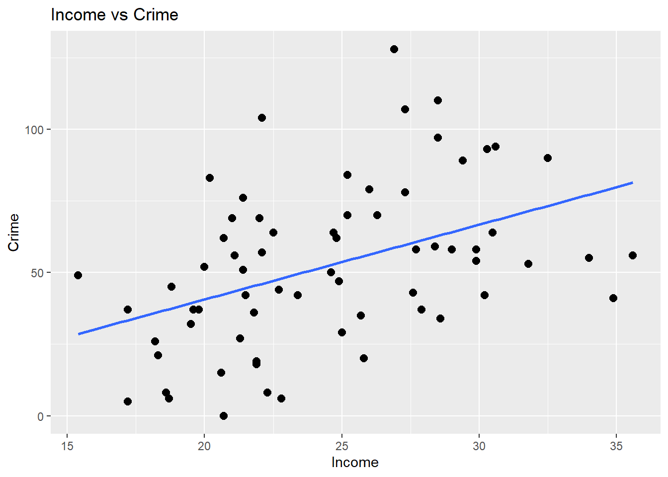
Figure 6.1: This graph shows how crime varies by income.
Looking at the slope line, the graph shows that as Income increases Crime also increases.
viz2 <- ggplot(florida_crime, aes(x=HighSchoolGrad, y=Crime))+
  geom_point(size=2.5)+
  geom_smooth(method = "lm", se=FALSE)+
  labs(
    title = "School vs Crime",
    x = "School",
    y = "Crime"
  )
print(viz2)
## `geom_smooth()` using formula = 'y ~ x'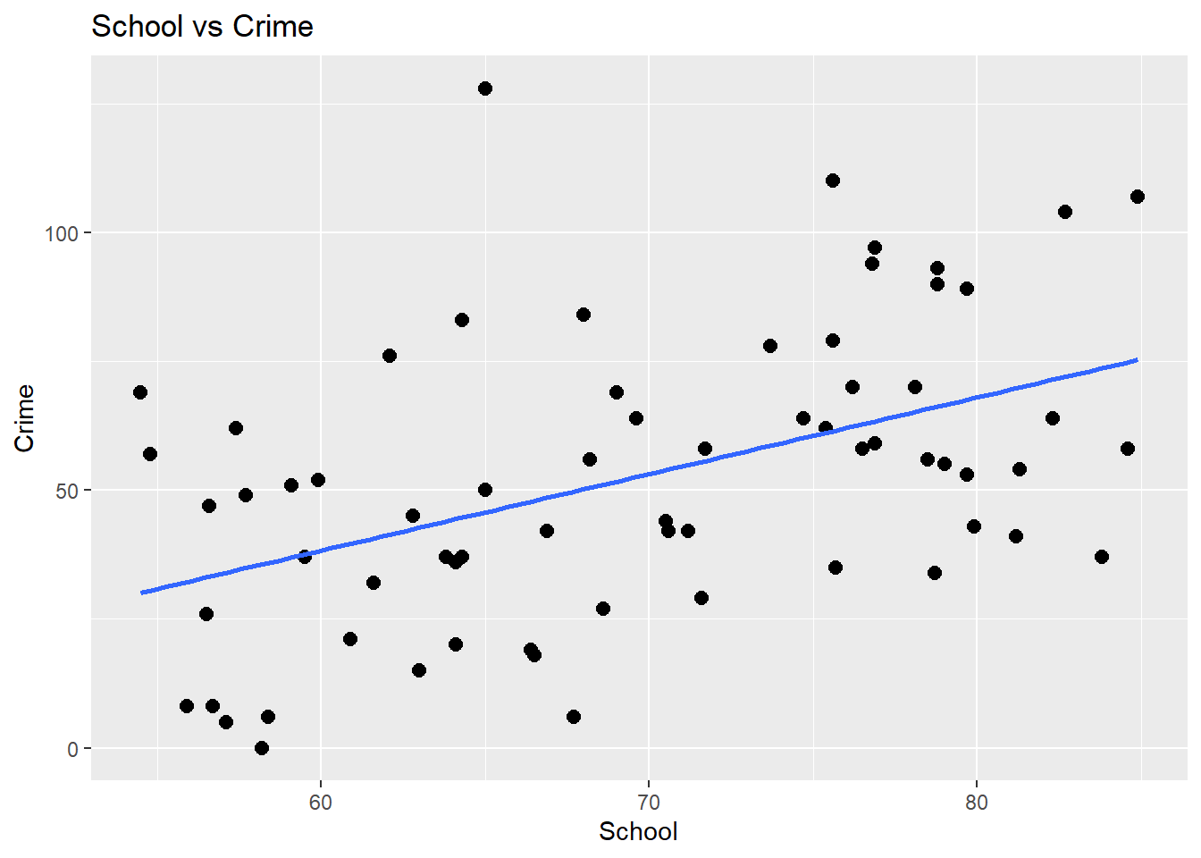
Figure 6.2: This graph shows hows crime varies by education.
Here we also see a similar trend from the previous graph. As school graduation increases so does Crime.
viz3 <- ggplot(florida_crime, aes(x=UrbanPop, y=Crime))+
  geom_point(size=2.5)+
  geom_smooth(method = "lm", se=FALSE)+
  labs(
    title = "Urban Lifestyle vs Crime",
    x = "UrbanPop",
    y = "Crime"
  )
print(viz3)
## `geom_smooth()` using formula = 'y ~ x'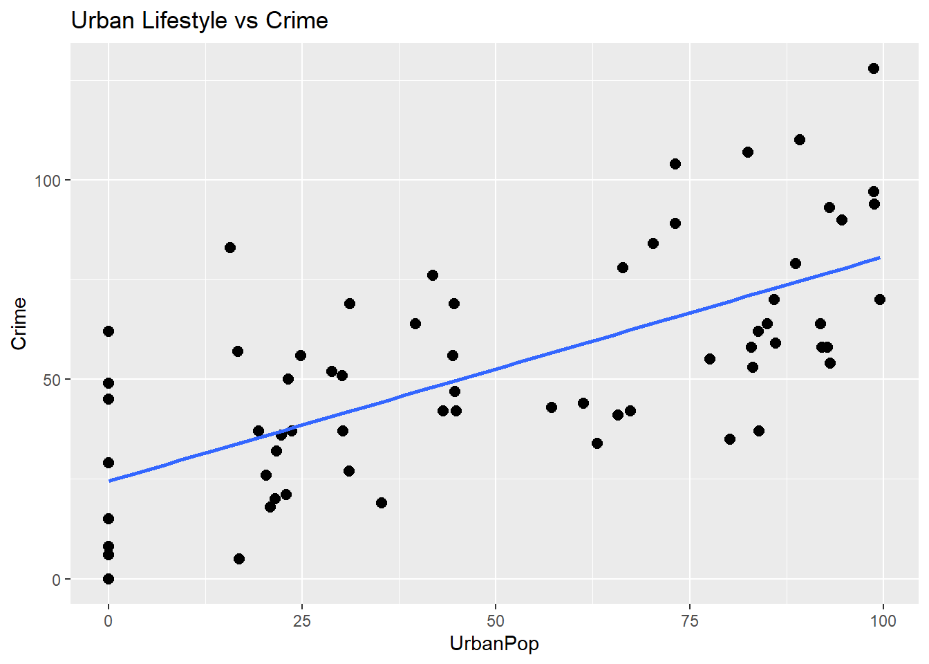
Figure 6.3: This graph shows how crime varies by population.
Again, there is a similar pattern as the two previous graphs. As the percentage of the urban population increases so does Crime.
Let’s use patchwork for better readability.
##
## Attaching package: 'patchwork'
## The following object is masked from 'package:MASS':
##
## area## `geom_smooth()` using formula = 'y ~ x'## `geom_smooth()` using formula = 'y ~ x'
## `geom_smooth()` using formula = 'y ~ x'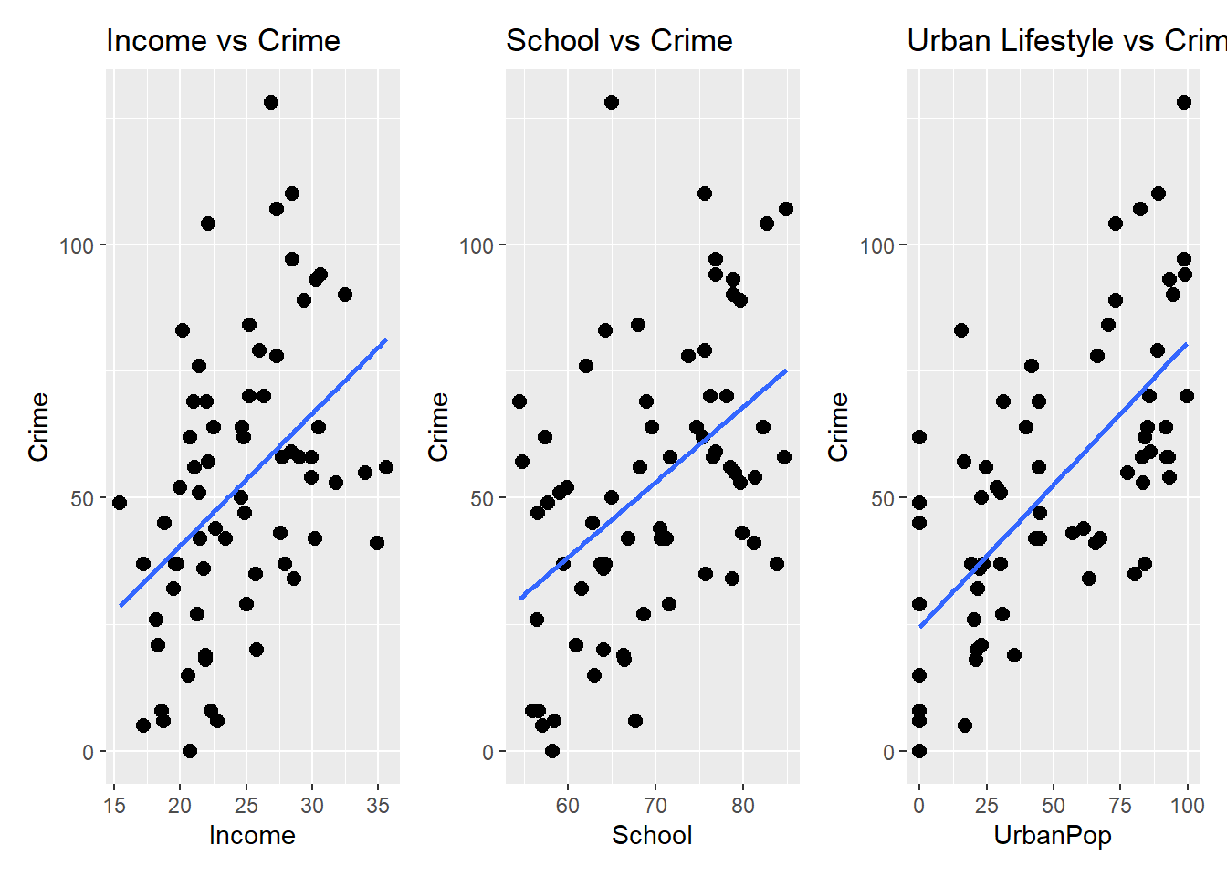
Figure 6.4: Side-by-side comparison of the three scatterplots.
6.4 Correlation Analysis
library(tidyverse)
Numeric_florida_crime <- florida_crime %>%
  dplyr::select(Crime, Income, HighSchoolGrad, UrbanPop)
head(Numeric_florida_crime)
## # A tibble: 6 × 4
## Crime Income HighSchoolGrad UrbanPop
## <dbl> <dbl> <dbl> <dbl>
## 1 104 22.1 82.7 73.2
## 2 20 25.8 64.1 21.5
## 3 64 24.7 74.7 85
## 4 50 24.6 65 23.2
## 5 64 30.5 82.3 91.9
## 6 94 30.6 76.8 98.9## Warning: package 'Hmisc' was built under R version 4.5.2##
## Attaching package: 'Hmisc'## The following objects are masked from 'package:dplyr':
##
## src, summarize## The following objects are masked from 'package:base':
##
## format.pval, units## Crime Income HighSchoolGrad UrbanPop
## Crime 1.00 0.43 0.47 0.68
## Income 0.43 1.00 0.79 0.73
## HighSchoolGrad 0.47 0.79 1.00 0.79
## UrbanPop 0.68 0.73 0.79 1.00
##
## n= 67
##
##
## P
## Crime Income HighSchoolGrad UrbanPop
## Crime 2e-04 0e+00 0e+00
## Income 2e-04 0e+00 0e+00
## HighSchoolGrad 0e+00 0e+00 0e+00
## UrbanPop 0e+00 0e+00 0e+00There is a positive correlation between Income and Crime r = 0.43 There is a positive correlation between HighSchoolGrad and Crime r= 0.47. There is a positive correlation between UrbanPop and Crime r = 0.68 (the strongest correlation among the variables).
6.5 Building Regression Models
##
## Call:
## lm(formula = Crime ~ Income, data = Numeric_florida_crime)
##
## Residuals:
##     Min      1Q  Median      3Q     Max
## -42.452 -21.347  -3.102  17.580  69.357
##
## Coefficients:
##             Estimate Std. Error t value Pr(>|t|)
## (Intercept) -11.6059    16.7863  -0.691 0.491782
## Income        2.6115     0.6729   3.881 0.000246 ***
## ---
## Signif. codes:  0 '***' 0.001 '**' 0.01 '*' 0.05 '.' 0.1 ' ' 1
##
## Residual standard error: 25.6 on 65 degrees of freedom
## Multiple R-squared:  0.1881, Adjusted R-squared:  0.1756
## F-statistic: 15.06 on 1 and 65 DF, p-value: 0.0002456## [1] 628.6045##
## Call:
## lm(formula = Crime ~ HighSchoolGrad, data = Numeric_florida_crime)
##
## Residuals:
## Min 1Q Median 3Q Max
## -43.74 -21.36 -4.82 17.42 82.27
##
## Coefficients:
## Estimate Std. Error t value Pr(>|t|)
## (Intercept) -50.8569 24.4507 -2.080 0.0415 *
## HighSchoolGrad 1.4860 0.3491 4.257 6.81e-05 ***
## ---
## Signif. codes: 0 '***' 0.001 '**' 0.01 '*' 0.05 '.' 0.1 ' ' 1
##
## Residual standard error: 25.12 on 65 degrees of freedom
## Multiple R-squared: 0.218, Adjusted R-squared: 0.206
## F-statistic: 18.12 on 1 and 65 DF, p-value: 6.806e-05## [1] 626.0932##
## Call:
## lm(formula = Crime ~ UrbanPop, data = Numeric_florida_crime)
##
## Residuals:
## Min 1Q Median 3Q Max
## -34.766 -16.541 -4.741 16.521 49.632
##
## Coefficients:
## Estimate Std. Error t value Pr(>|t|)
## (Intercept) 24.54125 4.53930 5.406 9.85e-07 ***
## UrbanPop 0.56220 0.07573 7.424 3.08e-10 ***
## ---
## Signif. codes: 0 '***' 0.001 '**' 0.01 '*' 0.05 '.' 0.1 ' ' 1
##
## Residual standard error: 20.9 on 65 degrees of freedom
## Multiple R-squared: 0.4588, Adjusted R-squared: 0.4505
## F-statistic: 55.11 on 1 and 65 DF, p-value: 3.084e-10## [1] 601.436.6 Multiple regression models
##
## Call:
## lm(formula = Crime ~ Income + UrbanPop, data = Numeric_florida_crime)
##
## Residuals:
##     Min      1Q  Median      3Q     Max
## -36.130 -15.590  -6.484  16.595  48.921
##
## Coefficients:
##             Estimate Std. Error t value Pr(>|t|)
## (Intercept)  39.9723    16.3536   2.444   0.0173 *
## Income       -0.7906     0.8049  -0.982   0.3297
## UrbanPop      0.6418     0.1110   5.784 2.36e-07 ***
## ---
## Signif. codes:  0 '***' 0.001 '**' 0.01 '*' 0.05 '.' 0.1 ' ' 1
##
## Residual standard error: 20.91 on 64 degrees of freedom
## Multiple R-squared:  0.4669, Adjusted R-squared:  0.4502
## F-statistic: 28.02 on 2 and 64 DF, p-value: 1.815e-09## [1] 602.4276##
## Call:
## lm(formula = Crime ~ Income + HighSchoolGrad, data = Numeric_florida_crime)
##
## Residuals:
## Min 1Q Median 3Q Max
## -42.75 -19.61 -4.57 18.52 77.86
##
## Coefficients:
## Estimate Std. Error t value Pr(>|t|)
## (Intercept) -46.1094 24.9723 -1.846 0.0695 .
## Income 1.0311 1.0839 0.951 0.3450
## HighSchoolGrad 1.0540 0.5729 1.840 0.0705 .
## ---
## Signif. codes: 0 '***' 0.001 '**' 0.01 '*' 0.05 '.' 0.1 ' ' 1
##
## Residual standard error: 25.14 on 64 degrees of freedom
## Multiple R-squared: 0.2289, Adjusted R-squared: 0.2048
## F-statistic: 9.5 on 2 and 64 DF, p-value: 0.000244## [1] 627.1524##
## Call:
## lm(formula = Crime ~ Income + UrbanPop + HighSchoolGrad, data = Numeric_florida_crime)
##
## Residuals:
## Min 1Q Median 3Q Max
## -35.407 -15.080 -6.588 16.178 50.125
##
## Coefficients:
## Estimate Std. Error t value Pr(>|t|)
## (Intercept) 59.7147 28.5895 2.089 0.0408 *
## Income -0.3831 0.9405 -0.407 0.6852
## UrbanPop 0.6972 0.1291 5.399 1.08e-06 ***
## HighSchoolGrad -0.4673 0.5544 -0.843 0.4025
## ---
## Signif. codes: 0 '***' 0.001 '**' 0.01 '*' 0.05 '.' 0.1 ' ' 1
##
## Residual standard error: 20.95 on 63 degrees of freedom
## Multiple R-squared: 0.4728, Adjusted R-squared: 0.4477
## F-statistic: 18.83 on 3 and 63 DF, p-value: 7.823e-09## [1] 603.67646.7 Comparing models
m1, R-squared of 0.188, Adjusted R-squared of 0.176, and AIC [628.6045] (variance explained is 18%).
m2, R-squared of 0.218, Adjusted R-squared of 0.206, and AIC [626.0932] (variance explained is 21%).
m3, R-squared of 0.459, Adjusted R-squared of 0.451, and AIC [601.43] (variance explained is 45%).
m4, R-squared of 0.467, Adjusted R-squared of 0.451, and AIC [602.4276] (variance explained is 45%).
m5, R-squared of 0.229, Adjusted R-squared of 0.205, and AIC [627.1524] (variance explained is 20%).
m6, R-squared of 0.473, Adjusted R-squared of 0.447, and AIC [603.6764] (variance explained is 45%).
6.8 Reflections
I can see that m3, m4, and m6 have the highest R-squared and Adjusted R-squared compared to m1,m2, and m5. Also, m3 has the lowest AIC which makes this model less complex when explaining the variance between the variables. I can also see that m4 and m6 have the lowest AIC following m3. m3 is more balance when it comes to R-squared and Adjusted R-squared. It’s safe to say that m3 is the best model for accuracy and simplicity.
6.9 Conclusion
After cleaning and analyzing the data by comparing different models for better crime predictions, I am confident about recommending model 3 (Crime and Urban Population) as it the most influential predictor when it comes to crime. This model explains 45% of the variance between the dependent variable (Crime) and the independent variable (UrbanPop). The PD should focus on highly populated areas to provide a sense of security to the population, which can help reduce the possibilities of committing crimes. One limitation is that correlation is not causation, and besides we don’t really have much data to look into age as a potential variable to understand what age groups are more likely to engage in such activities and devise better plans for interventions.