Code
rwb_map_2025 <- readRDS(paste0(here::here(), "/data/chap041/rwb_map_2025.rds"))
leaflet::leaflet(rwb_map_2025) |>
leaflet::addPolygons()August 21, 2025
Objectives
Learn making choropleth maps with {leaflet} /using my RWB data as practical example
The {leaflet} documentation transforms the step-by-step tutorial for leaflet.js into R code.
Instead of using the tutorial data I am working with my own RBW dataset. rbw_map_2925.rds is a {sf} data frame suitable to work with {leaflet} as I have already demonstrated with Graph 3.4.
For the basemap, the tutorial uses the same “mapbox.light” MapBox style that the leaflet.js example does. This requires a MapBox account, that I have already organized in a previous learning activity on map making.
During the registration process you get an access token that you have to put with a variable name into your .Renviron file. It is convention to use upper-case letter like MAPBOX_ACCESS_TOKEN.
But one can also just use leaflet::addTiles() in place of the leaflet::addProviderTiles() call, or choose a free provider.
Adding tiles in Leaflet refers to the process of overlaying a grid of small image tiles onto a map to create a background layer, which helps users orient themselves geographically. In my understanding I do not need adding tiles as background layers as I am using just colors for the choropleth maps. All other necessary information like borders (geometry column) or country labels (country_en column) are stored in the {sf} class of data frame.
R Code 4.1 : Most basic map from a {sf} data frame
rwb_map_2025 <- readRDS(paste0(here::here(), "/data/chap041/rwb_map_2025.rds"))
leaflet::leaflet(rwb_map_2025) |>
leaflet::addPolygons()It is interesting that {leaflet} centered the map automatically. I do not know if this feature depends on the exclusion of leaflet::setView() and/or leaflet::addTiles().
If I would have uses the standard leaflet::addTiles() the world view would be the same. But zooming into a region would bring up the OpenStreetMap default street map. (There are many different types of maps (King, n.d.).)
But to learn how to apply leaflet::addProviderTiles() I have used in the next code chunk the free OpenTopoMap from OpenStreetMap.
R Code 4.2 : Demo: World map with freely available OpenTopoMap tiles from OpenStreetMap
leaflet::leaflet(rwb_map_2025) |>
leaflet::setView(0, 45, 2) |>
leaflet::addProviderTiles(
"OpenTopoMap",
options = leaflet::tileOptions(noWrap = TRUE)
) |>
leaflet::addPolygons()OpenTopoMap tiles from OpenStreetMap
(The line options = leaflet::tileOptions(noWrap = TRUE) is explained in Section 4.1.2.2.2.)
Another — even more basic option — would be to use just leaflet::addTiles() instead of the line with leaflet::addProviderTiles(<provider name>).
In R Code 4.2 I have used specific leaflet::setView() in anticipation of appropriate arguments to center the map explained in the folowing section on ‘Area selection’.
The next problem for a nice choropleth map is to get the latitude and longitude data for an appropriate area selection fitting in the plotting bounding box. As I am using a world map I could try without these data, but it turned in Graph 3.4 out, that this is not a correct solution.
To get exact coordinates for any map I learned from another previous learning enterprise following an article and video by FelixAnalytix (2023b, 2023a) that OpenStreetMap has a nice tool to get the coordinates of a specific bounding box.
There are several options to get the coordinates of the bounding box for Leaflet.
(The next two paragraphs originate from the Brave-KI with the search string “r leaflet latitude and longitude for world center point”.)
The geographic center of the world is not a single, universally agreed-upon point, but a commonly referenced location is the intersection of the Prime Meridian (0° longitude) and the Equator (0° latitude), which is located in the Gulf of Guinea, off the western coast of Africa This point is often used as a reference for the world’s center in geographic and cartographic contexts.
In the R programming language, when using the {leaflet} package, the
leaflet::setView()function is used to center the map on a specific location by specifying the longitude and latitude. For the world center point, this would be set to longitude 0 and latitude 0. The {leaflet} package expects all point, line, and shape data to be specified in latitude and longitude using the WGS 84 coordinate reference system (EPSG:4326) For example, to center a map on the world’s center point, you would useleaflet::setView(lng = 0, lat = 0, zoom = 2)within aleaflet::leaflet()object.
R Code 4.3 : World map with centered 0 coordinates
0 coordinates using MapBox tiles
leaflet::leaflet(rwb_map_2025) |>
leaflet::setView(0, 0, 2) |>
leaflet::addProviderTiles(
"MapBox",
options = leaflet::providerTileOptions(
id = "mapbox.light",
accessToken = Sys.getenv('MAPBOX_ACCESS_TOKEN')
)
) |>
leaflet::addPolygons()As I have already noticed in the World tab of the Basic Map section, because of the height-width ratio a small correction of the north/south center point is necessary.
Although my RWB map does not contain Antarctica, the map is still too big. Previously (see World tab of the Basic Map section) I believed that it is just a mater of the heigt-width ratio of the figure. But now I think the situation is more complex:
Finding the best configuration to fit my plotting area depends on several interacting parameters:
lat and lng coordinates,Another important issue affecting the center coordinates is the omission of Antarctica in my world map!
As in Important 4.1 explained, it is difficult to understand the result of the different interacting factors. Therefore a bit of experimentation is always necessary.
R Code 4.4 : World map with theoretical and practical center coordinates
```{r}
#| label: fig-052-practical-center-coordinates
#| lst-label: lst-052-practical-center-coordinates
#| fig-cap: "World map centered after some experimentation with figure dimension, coordinates and Quarto layout. The markers show the difference between theoretical (0, 0) and practical (0, 45) center coordinates."
#| lst-cap: "World map centered after some experimentation showing theoretical (0, 0) and practical (0, 45) center coordinates"
#| fig-height: 8
#| fig-width: 7
leaflet::leaflet(rwb_map_2025) |>
leaflet::setView(0, 45, 2) |>
leaflet::addPolygons() |>
leaflet::addMarkers(0, 0, popup = 'Theretical center at 0,0') |>
leaflet::addMarkers(0, 45, popup = 'Practical center at 0,45')
```(The next two paragraphs originate from the Brave-KI with the search string “r leaflet bounding box for a world map”.)
A function can be created to calculate the bounding box based on the map’s center coordinates, zoom level, and the specified width and height of the map widget. This approach uses the formulae derived from Leaflet’s tile grid system, where the longitude width is calculated as
\[360 \times \text{width} / 2^{(\text{zoom} + 8)}\]
and the latitude height as
\[360 \times \text{height} \times \cos(\text{lat}/180 \times \pi) / 2^{(\text{zoom} + 8)}\]
The bounding box coordinates are then derived from the center point and these calculated extents This method is effective for maps with defined dimensions and a known zoom level, though accuracy can decrease at lower zoom levels.
The maximum bounds for the entire world in Leaflet are defined by the coordinates \([-90, -180]\) (southwest corner) and \([90, 180]\) (northeast corner), which represent the full range of latitude and longitude. To ensure the map displays only one instance of the world and prevents the display of duplicate world copies when panning, the
noWrapoption should be set totruewhen adding a tile layer, as I have done in Listing / Output 3.4.
I haven’t tested the pretty complicated calculation for the bounding box coordinates. It is easier to use the defined coordinates together with the noWrap option already used in Listing / Output 4.2.
R Code 4.5 : World map with bounding box
leaflet::leaflet(rwb_map_2025) |>
leaflet::setMaxBounds(-90, -180, 90, 180) |>
leaflet::addProviderTiles(
"OpenTopoMap",
options = leaflet::tileOptions(noWrap = TRUE)
) |>
leaflet::addPolygons()OpenTopoMap tiles from OpenStreetMap
Another strategy is to set the bounding box in OpenStreetMap manually as the following image shows:
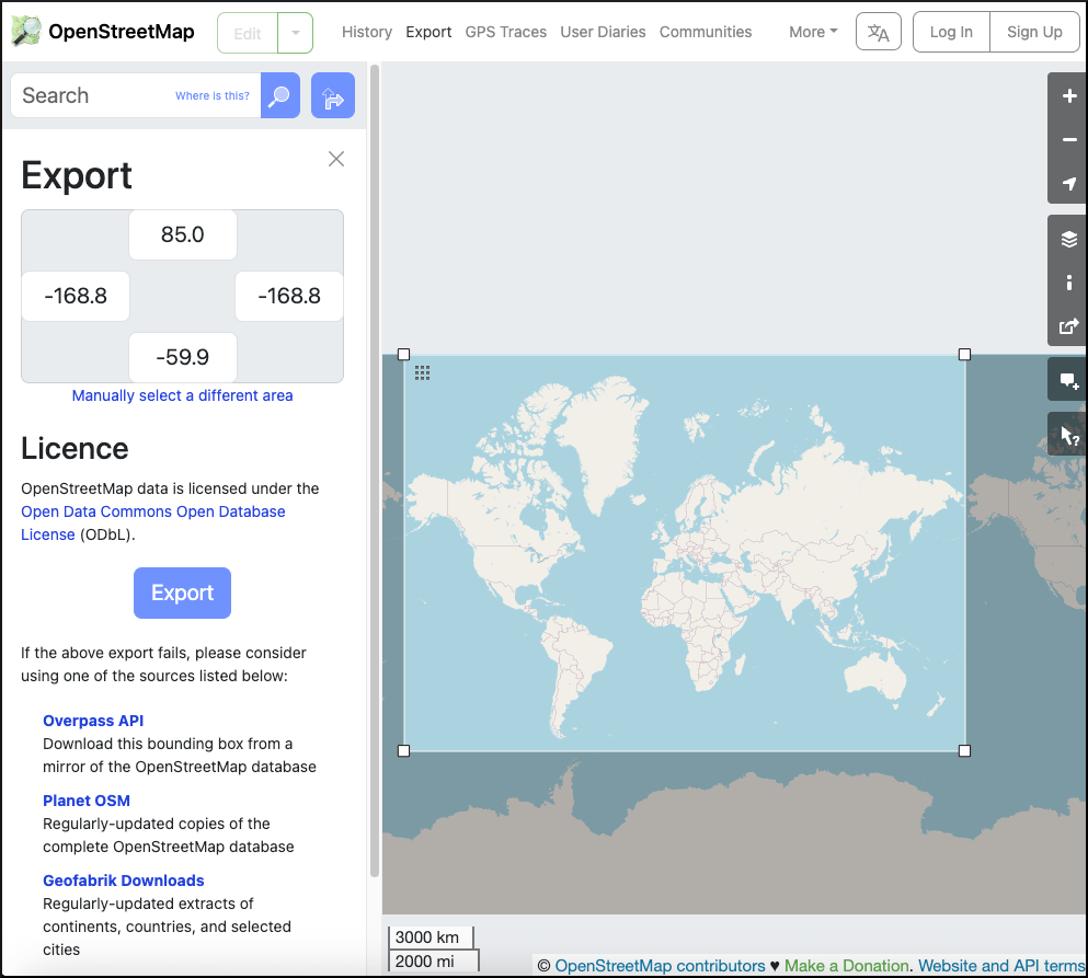
I have set the bounding area for a world map without Antarctica. I used the mouse to get the appropriate window on the right pane. The coordinates appear on the left side. The coordinates -59.9 / -168.8 (bottom, left) represent lat and lng of the bottom left point. 85.0 / -168.8 (top, right) are the coordinates for the top right point.
R Code 4.6 : Setting the bounding area manually with OpenStreetMap tool
leaflet::leaflet(rwb_map_2025) |>
leaflet::setMaxBounds(-60, -170, 85, 170) |>
leaflet::addProviderTiles(
"OpenTopoMap",
options = leaflet::tileOptions(noWrap = TRUE)
) |>
leaflet::addPolygons()The results from Listing / Output 4.6 and Listing / Output 4.5 are very similar as their values differ only few degrees. From the practical perspective to choose any region of the world only the last option (setting the boundaries manually) is viable.
Until now we have only use the default styling options for leaflet::addPolygons(). It resulted in dark blue thick country border lines and light blue background for the country areas.
An important part of spatial visualization is mapping variables to colors. While R has no shortage of built-in functionality to map values to colors, the {leaflet} developers found that there was enough friction in the process to warrant introducing some wrapper functions that do a lot of the work for you.
To that end, they’ve created a family of color*() convenience functions that can be used to easily generate palette functions. Essentially, you call the appropriate color function with
The color function returns a palette function that can be passed a vector of input values, and it’ll return a vector of colors in #RRGGBB(AA) format.
There are currently three color functions for dealing with continuous input: leaflet::colorNumeric(), leaflet::colorBin(), and leaflet::colorQuantile(); and one for categorical input, leaflet::colorFactor().
R Code 4.7 : Using leaflet::colorNumeric() to demonstrate the function results
leaflet::colorNumeric()
# Call the color function (colorNumeric) to create a new palette function
pal <- leaflet::colorNumeric(c("red", "green", "blue"), 1:100)
# Pass the palette function a data vector to get the corresponding colors
pal(c(1, 6, 9, 20, 25, 29, 30, 31, 40, 45, 60, 90, 100))#> [1] "#FF0000" "#F74A00" "#F15F00" "#D99400" "#CBA800" "#BEB700" "#BABB00"
#> [8] "#B7BE00" "#8EDD00" "#6AED00" "#66D663" "#644FDC" "#0000FF"To understand the effect of the code in Listing / Output 4.7 it is helpful to convert the resulting vector of colors from #RRGGBB(AA) format to the colors themselves:

The three palette colors (red, green, blue) are equally spaced through the domain (1 to 100). Depending of the actual data value, pal interpolates the values and spits out the appropriate color for this value. For instance in the example the range between red and green is 50, half of it (25) is a mixture between red and green. Low values are different shades of red, values started from the middle value 25 gets with their rising number greener until the reach the 50. From here the blue color wins increasing effect.
The four color functions all have two required arguments, palette and domain.
The palette argument specifies the colors to map the data to. This argument can take one of several forms:
grDevices::palette(), c("#000000", "#0000FF", "#FFFFFF"), grDevices::topo.colors(10).grDevices::colorRamp(c("#000000", "#FFFFFF"), interpolate="spline")
The domain argument tells the color function the range of input values. You can pass NULL here to create a palette function that doesn’t have a preset range; the range will be inferred from the data each time you invoke the palette function. If you use a palette function multiple times across different data, it’s important to provide a non-NULL value for domain so the scaling between data and colors is consistent.
The following graphics uses continuous colors to map continuous input. We will map the {sf} data frame rwb_map_20225 with its global score values of the WPFI directly to the “Blues” palette from Color Brewer 2. The “Blues” palette only contains nine colors, but leaflet::colorNumeric() interpolates these colors so we get continuous output.
c("white", "navy") or c("#FFFFFF", "#000080") for a similar effect. You can also pass more than two colors, for a diverging palette for example. And for maximum flexibility, you can even pass a function that takes a numeric value over the interval [0,1] and returns a color.leaflet::colorNumeric(), you can provide either the full range of the data, a min/max value (11.32 / 92.31) as in this example, or a set of numbers that leaflet::colorNumeric() can call range() on.range(countries$gdp_md_est) and return colors in "#RRGGBB" format.R Code 4.8 : Choropleth map with continuous colors for 2025 WPF Index
rwb_map_2025 <- readRDS(paste0(here::here(), "/data/chap041/rwb_map_2025.rds"))
# Create a continuous palette function
pal <- leaflet::colorNumeric( # (3)
palette = "Blues", # (1)
domain = rwb_map_2025$score) # (2)
leaflet::leaflet(rwb_map_2025) |>
leaflet::setView(0, 45, 2) |>
leaflet::addPolygons(
stroke = FALSE,
smoothFactor = 0.2,
fillOpacity = 1,
color = ~pal(score)
) |>
leaflet::addLegend(pal = pal, values = ~score, opacity = 0.7, title = NULL,
position = "bottomleft")To see the differences of the various map scales I needed to add a legend, a feature covered in detail in Section 4.1.6.
Compare Graph 2.1 with Graph 4.9. Keep in mind that Graph 4.9
But besides these differences both figures are quite similar.
Continuous input is mapped onto discrete colors with leaflet::colorBin() and leaflet::colorQuantile().
leaflet::colorBin() maps numeric input data to a fixed number of output colors using binning (slicing the input domain up by value).leaflet::colorQuantile() maps numeric input data to a fixed number of output colors using quantiles by slicing the input domain into subsets with equal numbers of observations.leaflet::colorBin() maps numeric input data to a fixed number of output colors using binning (slicing the input domain up by value). To divide input values into bins of equal range is only appropriate for variables with a uniform distribution and is not recommended for variables with a skewed distribution as the resulting map may end up having little color diversity.
You can specify either the exact breaks to use, or the desired number of bins. Note that in the latter case, if pretty = TRUE (the default) you’ll end up with nice round breaks but not necessarily the number of bins you wanted.
R Code 4.9 : Choropleth map with discrete colors for 2025 WPF Index
rwb_map_2025 <- readRDS(paste0(here::here(), "/data/chap041/rwb_map_2025.rds"))
labels <- sprintf(
"<strong>%s</strong><br/>score: %g",
rwb_map_2025$country_en, rwb_map_2025$score
) |> lapply(htmltools::HTML)
# Create a discrete palette function
binpal <- leaflet::colorBin(
palette = "Blues",
domain = rwb_map_2025$score,
bins = 15,
pretty = TRUE)
leaflet::leaflet(rwb_map_2025) |>
leaflet::setView(0, 45, 2) |>
leaflet::addPolygons(
stroke = FALSE,
smoothFactor = 0.5,
fillOpacity = 1,
color = ~binpal(score),
label = labels
) |>
leaflet::addLegend(pal = binpal, values = ~score, opacity = 0.7, title = NULL,
position = "bottomleft")#> Warning in RColorBrewer::brewer.pal(max(3, n), palette): n too large, allowed maximum for palette Blues is 9
#> Returning the palette you asked for with that many colors
#> Warning in RColorBrewer::brewer.pal(max(3, n), palette): n too large, allowed maximum for palette Blues is 9
#> Returning the palette you asked for with that many colors
#> Warning in RColorBrewer::brewer.pal(max(3, n), palette): n too large, allowed maximum for palette Blues is 9
#> Returning the palette you asked for with that many colorsI have use in Listing / Output 4.9 the pretty = TRUE argument, otherwise I would get very weird bins starting with 11.320-20.319 and ending with 83.311-92.310. In this case I get with pretty = TRUE not only nice boundaries but also the desired number of bins (nine).
leaflet::colorQuantile() maps numeric input data to a fixed number of output colors using quantiles (slicing the input domain into subsets with equal numbers of observations). This has the potential disadvantage that bin ranges can vary widely.
R Code 4.10 : Choropleth map with quantiled colors for 2025 WPF Index
rwb_map_2025 <- readRDS(paste0(here::here(), "/data/chap041/rwb_map_2025.rds"))
labels <- sprintf(
"<strong>%s</strong><br/>score: %g",
rwb_map_2025$country_en, rwb_map_2025$score
) |> lapply(htmltools::HTML)
# Create a discrete palette function
qpal <- leaflet::colorQuantile(
palette = "Blues",
domain = rwb_map_2025$score,
n = 9
)
leaflet::leaflet(rwb_map_2025) |>
leaflet::setView(0, 45, 2) |>
leaflet::addPolygons(
stroke = FALSE,
smoothFactor = 0.5,
fillOpacity = 1,
color = ~qpal(score),
label = labels
) |>
leaflet::addLegend(pal = qpal, values = ~score, opacity = 0.7, title = "Global score",
position = "bottomleft")Both discrete color scales (Listing / Output 4.9 and Listing / Output 4.10) are generally limited by the maximum number of palette colors. This in nine the case of “Blues”. If you override this maximum the program interpolated the colors with a warning message:
Warning in RColorBrewer::brewer.pal(max(3, n), palette) : n too large, allowed maximum for palette Blues is 9 Returning the palette you asked for with that many colors
For categorical data, use leaflet::colorFactor(). If the palette contains the same number of elements as there are factor levels, then the mapping will be 1:1; otherwise, the palette will be interpolated to produce the desired number of colors.
You can specify the input domain either by passing a factor or character vector to domain, or by providing levels directly using the levels parameter (in which case the domain will be ignored).
R Code 4.11 : Choropleth map with colors representing categories (factors) for the 2025 WPF Index
rwb_map_2025 <- readRDS(paste0(here::here(), "/data/chap041/rwb_map_2025.rds"))
rwb_colors <- c("#c6e269", "#ecc33d", "#e29950", "#de643a", "#9f1714" )
labels <- sprintf(
"<strong>%s</strong><br/>%s<br/>Score: %g",
rwb_map_2025$country_en, rwb_map_2025$score_situation, rwb_map_2025$score
) |> lapply(htmltools::HTML)
# Create a discrete palette function
factpal <- leaflet::colorFactor(
palette = rwb_colors,
domain = rwb_map_2025$score_situation,
levels = c("1. Good",
"2. Rather Good",
"3. Problematic",
"4. Difficult",
"5. Very Serious"
)
)
leaflet::leaflet(rwb_map_2025) |>
leaflet::setView(0, 45, 2) |>
leaflet::addPolygons(
fillColor = ~factpal(score_situation),
fillOpacity = 1,
smoothFactor = 0.5,
label = labels,
stroke = TRUE,
weight = 2,
opacity = 1,
color = "white",
dashArray = "3"
) |>
leaflet::addLegend(pal = factpal, values = ~score_situation, opacity = 1, title = "Score situation",
position = "bottomleft")The next thing we’ll want is to make the polygons highlight as the mouse passes over them. The leaflet::addPolygon() function has a highlight argument that makes this simple.
R Code 4.12 : Interactive choropleth map for the 2025 WPF Index
rwb_map_2025 <- readRDS(paste0(here::here(), "/data/chap041/rwb_map_2025.rds"))
rwb_colors <- c("#c6e269", "#ecc33d", "#e29950", "#de643a", "#9f1714" )
labels <- sprintf(
"<strong>%s</strong><br/>%s<br/>Score: %g",
rwb_map_2025$country_en, rwb_map_2025$score_situation, rwb_map_2025$score
) |> lapply(htmltools::HTML)
# Create a discrete palette function
factpal <- leaflet::colorFactor(
palette = rwb_colors,
domain = rwb_map_2025$score_situation,
levels = c("1. Good",
"2. Rather Good",
"3. Problematic",
"4. Difficult",
"5. Very Serious"
)
)
leaflet::leaflet(rwb_map_2025) |>
leaflet::setView(0, 45, 2) |>
leaflet::addPolygons(
fillOpacity = 1,
fillColor = ~factpal(score_situation),
smoothFactor = 0.5,
label = labels,
stroke = TRUE,
weight = 2,
opacity = 1,
color = "white",
dashArray = "3",
highlightOptions = leaflet::highlightOptions(
weight = 2,
color = "black",
dashArray = "",
fillOpacity = 1,
bringToFront = TRUE)
) |>
leaflet::addLegend(pal = factpal, values = ~score_situation, opacity = 1, title = NULL,
position = "bottomleft")(The Leaflet.js tutorial also adds an event handler that zooms into a state when it’s clicked. This isn’t currently possible with the {leaflet} R package, except with either custom JavaScript or using {shiny}, both of which are outside the scope of this example.)
Now let’s explain how to expose the state names and values to the user, as I already have done.
The Leaflet.js tutorial shows the hovered-over state’s information in a custom control. Again, that’s possible by adding custom JavaScript or using Shiny, but for this example we’ll use the built-in labels feature instead.
We’ll generate the labels by handcrafting some HTML, and passing it to base::lapply(htmltools::HTML) so that Leaflet knows to treat each label as HTML instead of as plain text. We’ll also set some label options to improve the style of the label element itself.
It is difficult to use popup information spread over several lines. The best general way is to use the base::stringf() function. base::paste() or base::cat() do not work.
Another way to display feature from the datasets using several lines is to apply the leafpop::popupTable() function of the {leafpop} package.
The advantage of base::stringf() is that you can adapt the popup string to your needs. With leafpop::popupTable() you have to stick with the name and content of the columns. But if you prepare the dataset to your needs then leafpop::popupTable() is way more comfortable to use.
R Code 4.13 : Interactive choropleth map for the 2025 WPF Index with popup info by mouse hovering
rwb_map_2025 <- readRDS(paste0(here::here(), "/data/chap041/rwb_map_2025.rds"))
rwb_colors <- c("#c6e269", "#ecc33d", "#e29950", "#de643a", "#9f1714" )
labels <- sprintf(
"<strong>%s</strong><br/>%s<br/>Score: %g",
rwb_map_2025$country_en, rwb_map_2025$score_situation, rwb_map_2025$score
) |> lapply(htmltools::HTML)
# Create a discrete palette function
factpal <- leaflet::colorFactor(
palette = rwb_colors,
domain = rwb_map_2025$score_situation,
levels = c("1. Good",
"2. Rather Good",
"3. Problematic",
"4. Difficult",
"5. Very Serious"
)
)
leaflet::leaflet(rwb_map_2025) |>
leaflet::setView(0, 45, 2) |>
leaflet::addPolygons(
fillOpacity = 1,
fillColor = ~factpal(score_situation),
smoothFactor = 0.5,
label = labels,
labelOptions = leaflet::labelOptions(
style = list("font-weight" = "normal", padding = "3px 8px"),
textsize = "15px",
direction = "auto"
),
stroke = TRUE,
weight = 2,
opacity = 1,
color = "white",
dashArray = "3",
highlightOptions = leaflet::highlightOptions(
weight = 2,
color = "black",
dashArray = "",
fillOpacity = 1,
bringToFront = TRUE)
) |>
leaflet::addLegend(pal = factpal, values = ~score_situation, opacity = 1, title = NULL,
position = "bottomleft")Listing / Output 4.13 contains the last version of the polygon layer.
As our final step, let’s add a legend. Because we chose to color our map using one of the color*() convenience functions, the leaflet::addLegend() function makes it particularly easy to add a legend with the correct colors and intervals.
I have this already done in Listing / Output 4.8 and the following code chunks. Here I will display the last version of the polygon layer as in Listing / Output 4.13 but for the continuous color scale.
R Code 4.14 : Choropleth map with continuous color scale with legend and all the other explained features
rwb_map_2025 <- readRDS(paste0(here::here(), "/data/chap041/rwb_map_2025.rds"))
labels <- sprintf(
"<strong>%s</strong><br/>score: %g",
rwb_map_2025$country_en, rwb_map_2025$score
) |> lapply(htmltools::HTML)
pal <- leaflet::colorNumeric(
palette = "Blues",
domain = rwb_map_2025$score)
leaflet::leaflet(rwb_map_2025) |>
leaflet::setView(0, 45, 2) |>
leaflet::addPolygons(
fillOpacity = 1,
fillColor = ~pal(score),
smoothFactor = 0.5,
label = labels,
labelOptions = leaflet::labelOptions(
style = list("font-weight" = "normal", padding = "3px 8px"),
textsize = "15px",
direction = "auto"
),
stroke = TRUE,
weight = 2,
opacity = 1,
color = "white",
dashArray = "3",
highlightOptions = leaflet::highlightOptions(
weight = 2,
color = "black",
dashArray = "",
fillOpacity = 1,
bringToFront = TRUE)
) |>
leaflet::addLegend(pal = pal, values = ~score, opacity = 1, title = "Global score",
position = "bottomleft")| term | definition |
|---|---|
| Choropleth | A choropleth map is a type of thematic map that uses shading or coloring to represent statistical data across predefined geographic regions. These regions can be political boundaries, such as states or countries, or natural divisions. Each area is colored based on the value of the variable being represented, typically using a gradient where darker shades indicate higher values and lighter shades indicate lower values. This visualization technique helps viewers quickly grasp patterns and trends within the dataset. It is important to note that choropleth maps can sometimes lead to misinterpretation due to the bias introduced by the size of the regions. Larger regions may appear to have more significance simply because of their size, even if their data values are the same as smaller regions. In this case use Cartograms. |
| CRS | A Coordinate Reference System (CRS) defines how locations on the Earth’s surface are represented in a two-dimensional plane. This is essential for accurate mapping and spatial analysis. CRSs are often defined using the PROJ.4 notation, which is a standard way to describe coordinate systems. CRSs can also be identified using EPSG codes, which are unique identifiers for different coordinate systems. |
| OpenStreetMap | OpenStreetMap (OSM) is a free, editable, and open-source map of the entire world, created and maintained by a global community of volunteers. It functions like a "Wikipedia of maps," allowing anyone to contribute, edit, and use the geospatial data, which includes information on roads, buildings, points of interest, land use, and more. The data is freely licensed under the Open Database License (ODbL), enabling its use for a wide range of purposes, including commercial applications, humanitarian efforts, and academic research, as long as proper attribution is given. |
| RWB | Reporters Without Borders (RWB), known by its French name Reporters sans frontières and acronym RSF, is an international non-profit and non-governmental organization headquartered in Paris, France, founded in 1985 in Montpellier by journalists Robert Ménard, Rémy Loury, Jacques Molénat, and Émilien Jubineau. It is dedicated to safeguarding the right to freedom of information and defends journalists and media personnel who are imprisoned, persecuted, or at risk for their work. The organization has consultative status at the United Nations, UNESCO, the Council of Europe, and the International Organisation of the Francophonie. |
| WPFI | The World Press Freedom Index (WPFI) is an annual ranking of countries compiled and published by Reporters Without Borders (RSF), an international non-governmental organization based in France, since 2002. It aims to reflect the degree of freedom that journalists, news organizations, and netizens have in each country, as well as the efforts made by authorities to respect this freedom. The index ranks 180 countries and territories based on RSF's assessment of their press freedom records in the preceding year. |
Session Info
xfun::session_info()#> R version 4.5.1 (2025-06-13)
#> Platform: aarch64-apple-darwin20
#> Running under: macOS Sequoia 15.6.1
#>
#> Locale: en_US.UTF-8 / en_US.UTF-8 / en_US.UTF-8 / C / en_US.UTF-8 / en_US.UTF-8
#>
#> Package version:
#> askpass_1.2.1 base64enc_0.1.3 bslib_0.9.0
#> cachem_1.1.0 class_7.3-23 classInt_0.4-11
#> cli_3.6.5 commonmark_2.0.0 compiler_4.5.1
#> cpp11_0.5.2 crosstalk_1.2.2 curl_7.0.0
#> DBI_1.2.3 digest_0.6.37 e1071_1.7-16
#> evaluate_1.0.5 farver_2.1.2 fastmap_1.2.0
#> fontawesome_0.5.3 fs_1.6.6 glossary_1.0.0
#> glue_1.8.0 graphics_4.5.1 grDevices_4.5.1
#> grid_4.5.1 here_1.0.1 highr_0.11
#> htmltools_0.5.8.1 htmlwidgets_1.6.4 httr_1.4.7
#> jquerylib_0.1.4 jsonlite_2.0.0 kableExtra_1.4.0
#> KernSmooth_2.23-26 knitr_1.50 labeling_0.4.3
#> lattice_0.22.7 lazyeval_0.2.2 leaflet_2.2.2
#> leaflet.providers_2.0.0 lifecycle_1.0.4 litedown_0.7
#> magrittr_2.0.3 markdown_2.0 MASS_7.3.65
#> memoise_2.0.1 methods_4.5.1 mime_0.13
#> openssl_2.3.3 pillar_1.11.0 pkgconfig_2.0.3
#> png_0.1.8 proxy_0.4-27 R6_2.6.1
#> rappdirs_0.3.3 raster_3.6.32 RColorBrewer_1.1-3
#> Rcpp_1.1.0 renv_1.1.5 rlang_1.1.6
#> rmarkdown_2.29 rprojroot_2.1.1 rstudioapi_0.17.1
#> rversions_2.1.2 rvest_1.0.5 s2_1.1.9
#> sass_0.4.10 scales_1.4.0 selectr_0.4.2
#> sf_1.0-21 sp_2.2.0 stats_4.5.1
#> stringi_1.8.7 stringr_1.5.1 svglite_2.2.1
#> sys_3.4.3 systemfonts_1.2.3 terra_1.8.60
#> textshaping_1.0.1 tibble_3.3.0 tinytex_0.57
#> tools_4.5.1 units_0.8-7 utf8_1.2.6
#> utils_4.5.1 vctrs_0.6.5 viridisLite_0.4.2
#> wk_0.9.4 xfun_0.53 xml2_1.4.0
#> yaml_2.3.10