
Chapter 7 Assignment 7 - Wage Analytics – Predicting High vs Low Earners Using Logistic Regression
7.1 Introduction
The Wage Analytics Division (WAD) has hired me as their new Data Scientist. My assignment is to determine whether demographic and employment characteristics can be used to predict whether a worker earns a high or low wage.
Using the Wage dataset from the ISLR package, I will create a binary wage category, explore statistical relationships between variables, and build a logistic regression model capable of predicting wage level using demographic, job, and health-related information.
My analysis will help the company understand which characteristics are associated with higher earnings and evaluate how well a predictive model performs on unseen data.
7.2 Step 1 – Create the WageCategory Variable
| year | age | maritl | race | education | region | jobclass | health | health_ins | logwage | wage | |
|---|---|---|---|---|---|---|---|---|---|---|---|
| 231655 | 2006 | 18 | 1. Never Married | 1. White | 1. < HS Grad | 2. Middle Atlantic | 1. Industrial | 1. <=Good | 2. No | 4.318063 | 75.04315 |
| 86582 | 2004 | 24 | 1. Never Married | 1. White | 4. College Grad | 2. Middle Atlantic | 2. Information | 2. >=Very Good | 2. No | 4.255273 | 70.47602 |
| 161300 | 2003 | 45 | 2. Married | 1. White | 3. Some College | 2. Middle Atlantic | 1. Industrial | 1. <=Good | 1. Yes | 4.875061 | 130.98218 |
| 155159 | 2003 | 43 | 2. Married | 3. Asian | 4. College Grad | 2. Middle Atlantic | 2. Information | 2. >=Very Good | 1. Yes | 5.041393 | 154.68529 |
| 11443 | 2005 | 50 | 4. Divorced | 1. White | 2. HS Grad | 2. Middle Atlantic | 2. Information | 1. <=Good | 1. Yes | 4.318063 | 75.04315 |
median_wage<- median(Wage$wage)

Wage <- Wage %>% mutate(
    WageCategory = case_when(
      wage > median_wage ~ "High",
      wage <= median_wage ~ "Low"),
    WageCategory = as.factor(WageCategory)
  )

Wage %>% head(n=5) %>% kable(caption = "Wage Dataset Including Wage Category (first 5 rows)")| year | age | maritl | race | education | region | jobclass | health | health_ins | logwage | wage | WageCategory | |
|---|---|---|---|---|---|---|---|---|---|---|---|---|
| 231655 | 2006 | 18 | 1. Never Married | 1. White | 1. < HS Grad | 2. Middle Atlantic | 1. Industrial | 1. <=Good | 2. No | 4.318063 | 75.04315 | Low |
| 86582 | 2004 | 24 | 1. Never Married | 1. White | 4. College Grad | 2. Middle Atlantic | 2. Information | 2. >=Very Good | 2. No | 4.255273 | 70.47602 | Low |
| 161300 | 2003 | 45 | 2. Married | 1. White | 3. Some College | 2. Middle Atlantic | 1. Industrial | 1. <=Good | 1. Yes | 4.875061 | 130.98218 | High |
| 155159 | 2003 | 43 | 2. Married | 3. Asian | 4. College Grad | 2. Middle Atlantic | 2. Information | 2. >=Very Good | 1. Yes | 5.041393 | 154.68529 | High |
| 11443 | 2005 | 50 | 4. Divorced | 1. White | 2. HS Grad | 2. Middle Atlantic | 2. Information | 1. <=Good | 1. Yes | 4.318063 | 75.04315 | Low |
7.3 Step 2 – Data Cleaning
##  [1] "year"         "age"          "maritl"       "race"         "education"
##  [6] "region"       "jobclass"     "health"       "health_ins"   "logwage"
## [11] "wage"         "WageCategory"
Wage <- Wage %>%
mutate(
across(
c("maritl", "race", "education", "region", "jobclass", "health", "health_ins"),
~substring(.x, 4)
)
)
Wage %>% head(n=5) %>% kable(caption = "Cleaned Wage Dataset (first 5 rows)")| year | age | maritl | race | education | region | jobclass | health | health_ins | logwage | wage | WageCategory | |
|---|---|---|---|---|---|---|---|---|---|---|---|---|
| 231655 | 2006 | 18 | Never Married | White | < HS Grad | Middle Atlantic | Industrial | <=Good | No | 4.318063 | 75.04315 | Low |
| 86582 | 2004 | 24 | Never Married | White | College Grad | Middle Atlantic | Information | >=Very Good | No | 4.255273 | 70.47602 | Low |
| 161300 | 2003 | 45 | Married | White | Some College | Middle Atlantic | Industrial | <=Good | Yes | 4.875061 | 130.98218 | High |
| 155159 | 2003 | 43 | Married | Asian | College Grad | Middle Atlantic | Information | >=Very Good | Yes | 5.041393 | 154.68529 | High |
| 11443 | 2005 | 50 | Divorced | White | HS Grad | Middle Atlantic | Information | <=Good | Yes | 4.318063 | 75.04315 | Low |
7.4 Step 3 – Classical Statistical Tests
7.4.1 A) T-Test
##
##  Welch Two Sample t-test
##
## data:  age by WageCategory
## t = 10.888, df = 2855, p-value < 2.2e-16
## alternative hypothesis: true difference in means between group High and group Low is not equal to 0
## 95 percent confidence interval:
##  3.681416 5.298535
## sample estimates:
## mean in group High  mean in group Low
##           44.68510           40.19512
Mean age for high earners: 45 years old
Mean age for low earners: 40 years old
t-statistic: 10.9
df: 2855
p-value < 2.2e-16
Age seems to differ between high earners and low earners. We have a high t-statistic and a very small p-value, suggesting that we are very confident in a large difference between the ages in both wage categories.
7.4.2 B) ANOVA
| education | min | Q1 | median | Q3 | max | mean | sd | n | missing |
|---|---|---|---|---|---|---|---|---|---|
| Advanced Degree | 38.60591 | 117.14682 | 141.77517 | 171.49763 | 318.3424 | 150.91778 | 53.90421 | 426 | 0 |
| College Grad | 32.36641 | 99.68946 | 118.88436 | 143.13494 | 281.7460 | 124.42791 | 41.18907 | 685 | 0 |
| Some College | 20.08554 | 89.24288 | 104.92151 | 121.38842 | 314.3293 | 107.75557 | 32.47473 | 650 | 0 |
| HS Grad | 23.27470 | 77.94638 | 94.07271 | 109.83399 | 318.3424 | 95.78335 | 28.56756 | 971 | 0 |
| < HS Grad | 20.93438 | 70.26177 | 81.28325 | 97.49329 | 152.2168 | 84.10441 | 21.57805 | 268 | 0 |
fig.cap = "This table shows preliminary descriptive statistics such as averages and frequencies so that we can better understand our dataset and what patterns to explore regarding wage and education."
anova_model_ed<- aov(wage ~ education, data = Wage)
summary(anova_model_ed)
## Df Sum Sq Mean Sq F value Pr(>F)
## education 4 1226364 306591 229.8 <2e-16 ***
## Residuals 2995 3995721 1334
## ---
## Signif. codes: 0 '***' 0.001 '**' 0.01 '*' 0.05 '.' 0.1 ' ' 1## Analysis of Variance Table (Type III SS)
## Model: wage ~ education
##
## SS df MS F PRE p
## ----- --------------- | ----------- ---- ---------- ------- ----- -----
## Model (error reduced) | 1226364.485 4 306591.121 229.806 .2348 .0000
## Error (from model) | 3995721.285 2995 1334.131
## ----- --------------- | ----------- ---- ---------- ------- ----- -----
## Total (empty model) | 5222085.770 2999 1741.276F-statistic: 229.81
df: 2999
p-value < 2e-16
With a very large F-statistic and a very small p-value, we can conclude that the variation in wages between education levels is statistically significant. Also, our PRE tells us that education level accounts for 23% of variance in wages.
7.4.3 C) Chi-Square/Association Test
| High | Low | |
|---|---|---|
| Asian | 113 | 77 |
| Black | 102 | 191 |
| Other | 9 | 28 |
| White | 1259 | 1221 |
fig.cap = "This figure is a contingency table representing the number of people in each wage category grouped by race."

Wage$race<- as.factor(Wage$race)
str(Wage$race)
## Factor w/ 4 levels "Asian","Black",..: 4 4 4 1 4 4 3 1 2 4 ...##
## Chi-square test of categorical association
##
## Variables: WageCategory, race
##
## Hypotheses:
## null: variables are independent of one another
## alternative: some contingency exists between variables
##
## Observed contingency table:
## race
## WageCategory Asian Black Other White
## High 113 102 9 1259
## Low 77 191 28 1221
##
## Expected contingency table under the null hypothesis:
## race
## WageCategory Asian Black Other White
## High 93.9 145 18.3 1226
## Low 96.1 148 18.7 1254
##
## Test results:
## X-squared statistic: 43.814
## degrees of freedom: 3
## p-value: <.001
##
## Other information:
## estimated effect size (Cramer's v): 0.121χ²: 43.8
df: 3
p-value < 0.001
Cramer’s V: 0.121
When comparing our observed and expected values, we see that White people performed as expected. A slightly higher number of Asian people earned higher wages than expected, and a slightly higher number of Black people earned lower wages than expected. Additionally, those who marked their race as “Other” tended to earn less than expected.
With a large chi-squared value and a small p-value, we can conclude that the relationship between race and wage category is statistically significant. However, with such a small effect size, the relationship is weak and we cannot assume that race itself plays much of a role in determining wage category.
7.5 Step 4 – Logistic Regression Model
7.5.3 Logistic Regression Output
##
## Call:
## glm(formula = WageCategory ~ age + maritl + race + education +
##     jobclass + health + health_ins, family = "binomial", data = training_data)
##
## Coefficients:
##                           Estimate Std. Error z value Pr(>|z|)
## (Intercept)               3.969497   0.449412   8.833  < 2e-16 ***
## age                      -0.019159   0.005179  -3.699 0.000216 ***
## maritlMarried            -0.880983   0.198852  -4.430 9.41e-06 ***
## maritlNever Married       0.382638   0.235167   1.627 0.103718
## maritlSeparated          -0.493750   0.445580  -1.108 0.267815
## maritlWidowed            -0.702502   0.641162  -1.096 0.273224
## raceBlack                 0.308966   0.280923   1.100 0.271407
## raceOther                 0.024598   0.587975   0.042 0.966630
## raceWhite                -0.163411   0.226615  -0.721 0.470850
## educationAdvanced Degree -2.727178   0.262521 -10.388  < 2e-16 ***
## educationCollege Grad    -1.918224   0.229754  -8.349  < 2e-16 ***
## educationHS Grad         -0.537104   0.218967  -2.453 0.014171 *
## educationSome College    -1.253153   0.226653  -5.529 3.22e-08 ***
## jobclassInformation      -0.239335   0.107600  -2.224 0.026128 *
## health>=Very Good        -0.305837   0.117671  -2.599 0.009347 **
## health_insYes            -1.208890   0.118014 -10.244  < 2e-16 ***
## ---
## Signif. codes:  0 '***' 0.001 '**' 0.01 '*' 0.05 '.' 0.1 ' ' 1
##
## (Dispersion parameter for binomial family taken to be 1)
##
##     Null deviance: 2910.9  on 2099  degrees of freedom
## Residual deviance: 2225.0  on 2084  degrees of freedom
## AIC: 2257
##
## Number of Fisher Scoring iterations: 4
7.5.4 Odds Ratio
##              (Intercept)                      age            maritlMarried
##              52.95789941               0.98102322               0.41437526
##      maritlNever Married          maritlSeparated            maritlWidowed
##               1.46614683               0.61033309               0.49534462
##                raceBlack                raceOther                raceWhite
##               1.36201634               1.02490299               0.84924198
## educationAdvanced Degree    educationCollege Grad         educationHS Grad
##               0.06540362               0.14686760               0.58443835
##    educationSome College      jobclassInformation        health>=Very Good
##               0.28560285               0.78715143               0.73650656
##            health_insYes
##               0.29852856
The predictors that matter most in predicting wage category is age, marital status, education, and health insurance status. Specifically, being older, married, having some college experience, a college degree, or an advanced degree, and having health insurance makes someone much less likely to earn a lower wage. Because of the fact that my model considers the positive outcome to be “Low” wage, all of these specific factors have a negative relationship with wage category (meaning they are more likely to earn a higher wage).
Having an advanced degree had the strongest effect on predicting higher wage, followed by having a college degree, then some college experience, then having active health insurance, being married, and finally older age with the smallest (but still statistically significant) effect size.
Health insurance status surprised me the most - not that it is shocking that people with higher wages tend to have health insurance, but it seems like (in my experience) many lower wage jobs still offer some sort of health insurance, If anything, I thought that it would have been a very weak predictor compared to the other variables.
7.6 Step 5 – Model Evaluation on Test Data
## fitting null model for pseudo-r2## McFadden
## 0.2356458This score tells us that our model has a good fit.
##                              Overall
## educationAdvanced Degree 10.38841873
## health_insYes            10.24365057
## educationCollege Grad     8.34903942
## educationSome College     5.52894400
## maritlMarried             4.43035351
## age                       3.69944093
## health>=Very Good         2.59909015
## educationHS Grad          2.45290419
## jobclassInformation       2.22430943
## maritlNever Married       1.62708918
## maritlSeparated           1.10810734
## raceBlack                 1.09982714
## maritlWidowed             1.09566872
## raceWhite                 0.72109599
## raceOther                 0.04183507
Education (namely College Grad & Advanced Degree) and health insurance are the strongest predictors of having a higher wage.
##                GVIF Df GVIF^(1/(2*Df))
## age        1.226363  1        1.107413
## maritl     1.230025  4        1.026217
## race       1.088403  3        1.014219
## education  1.171092  4        1.019938
## jobclass   1.076950  1        1.037762
## health     1.057935  1        1.028560
## health_ins 1.020670  1        1.010282
Thankfully, our model shows no colinearity.
7.6.1 Predicted Probabilities & Classes
test_data$pred_prob <- predict(train_model, newdata = test_data, type = "response")
test_data$pred_class <- ifelse(test_data$pred_prob > 0.5, "Low", "High") %>% as.factor()
test_data %>% head(n=10) %>% kable(caption = "Predicted Probabilities and Classes (first 10 rows)")| year | age | maritl | race | education | region | jobclass | health | health_ins | logwage | wage | WageCategory | pred_prob | pred_class | |
|---|---|---|---|---|---|---|---|---|---|---|---|---|---|---|
| 231655 | 2006 | 18 | Never Married | White | < HS Grad | Middle Atlantic | Industrial | <=Good | No | 4.318063 | 75.04315 | Low | 0.9790380 | Low |
| 86582 | 2004 | 24 | Never Married | White | College Grad | Middle Atlantic | Information | >=Very Good | No | 4.255273 | 70.47602 | Low | 0.7799730 | Low |
| 376662 | 2008 | 54 | Married | White | College Grad | Middle Atlantic | Information | >=Very Good | Yes | 4.845098 | 127.11574 | High | 0.1440839 | High |
| 450601 | 2009 | 44 | Married | Other | Some College | Middle Atlantic | Industrial | >=Very Good | Yes | 5.133021 | 169.52854 | High | 0.3780648 | High |
| 305706 | 2007 | 34 | Married | White | HS Grad | Middle Atlantic | Industrial | >=Very Good | No | 4.397940 | 81.28325 | Low | 0.8070183 | Low |
| 160191 | 2003 | 37 | Never Married | Asian | College Grad | Middle Atlantic | Industrial | >=Very Good | No | 4.414973 | 82.67964 | Low | 0.8052107 | Low |
| 230312 | 2006 | 50 | Married | White | Advanced Degree | Middle Atlantic | Information | >=Very Good | No | 5.360552 | 212.84235 | High | 0.2132905 | High |
| 301585 | 2007 | 56 | Married | White | College Grad | Middle Atlantic | Industrial | <=Good | Yes | 4.861026 | 129.15669 | High | 0.2184157 | High |
| 158226 | 2003 | 38 | Married | Asian | College Grad | Middle Atlantic | Information | >=Very Good | No | 5.301030 | 200.54326 | High | 0.4742904 | High |
| 448410 | 2009 | 75 | Married | White | College Grad | Middle Atlantic | Industrial | >=Very Good | Yes | 4.447158 | 85.38394 | Low | 0.1251232 | High |
7.6.2 Confusion Matrix
conf_matrix <- confusionMatrix(test_data$pred_class, test_data$WageCategory, positive = "Low")
conf_matrix
## Confusion Matrix and Statistics
##
## Reference
## Prediction High Low
## High 310 116
## Low 135 339
##
## Accuracy : 0.7211
## 95% CI : (0.6906, 0.7502)
## No Information Rate : 0.5056
## P-Value [Acc > NIR] : <2e-16
##
## Kappa : 0.4419
##
## Mcnemar's Test P-Value : 0.2559
##
## Sensitivity : 0.7451
## Specificity : 0.6966
## Pos Pred Value : 0.7152
## Neg Pred Value : 0.7277
## Prevalence : 0.5056
## Detection Rate : 0.3767
## Detection Prevalence : 0.5267
## Balanced Accuracy : 0.7208
##
## 'Positive' Class : Low
## - Accuracy: 0.72
- The model accurately predicted the correct wage category 72% of the time.
- Sensitivity: 0.75
- The model accurately predicted low wage earners 75% of the time.
- Specificity: 0.70
- The model accurately predicted high earners 70% of the time.
- Balanced Accuracy: 0.72
- Our balanced accuracy shows us that our observed data is likely pretty balanced, since the balanced accuracy rate is the same as our regular accuracy rate. When we run table(Wage$WageCategory), we can see that our data is very balanced (~1500 per category).
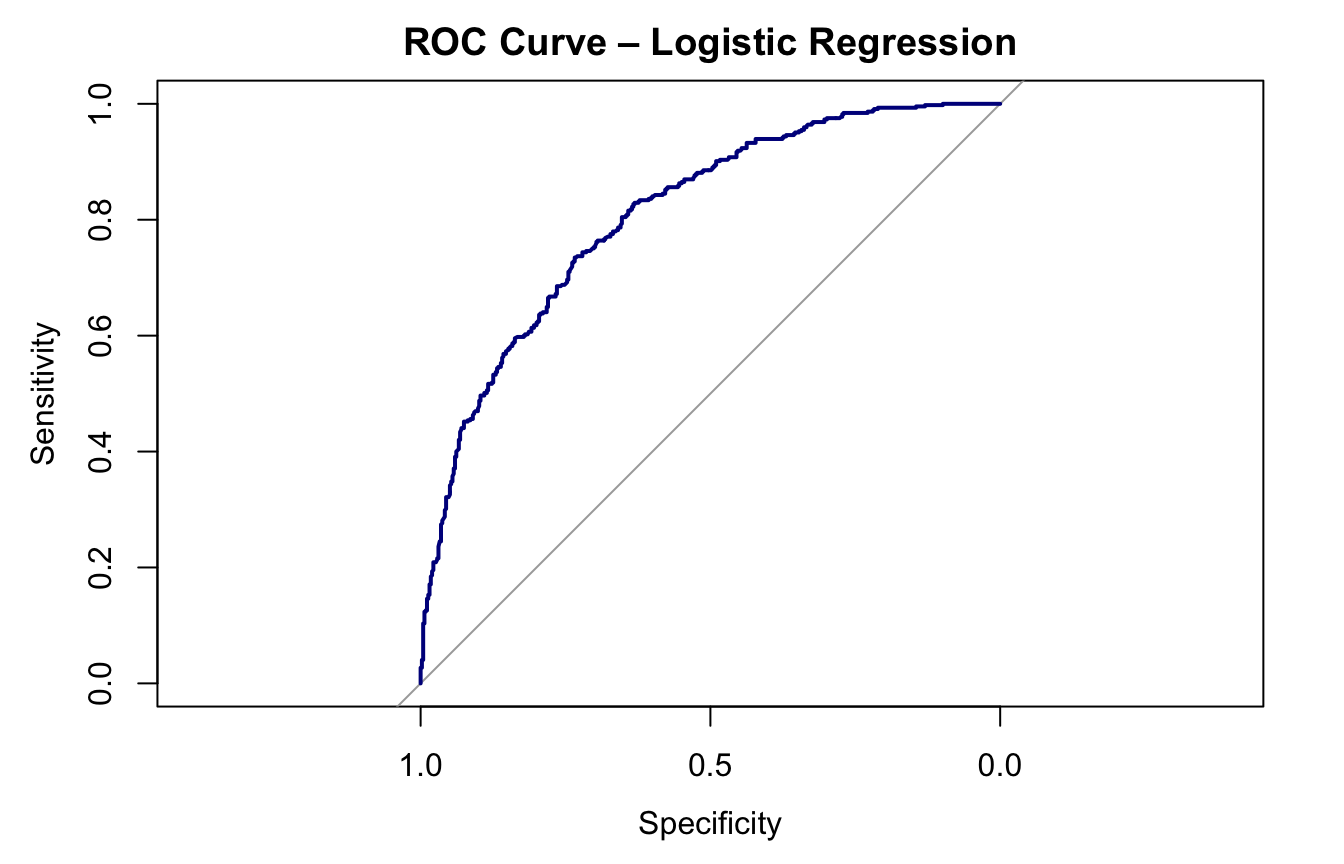
7.6.4 Area Under the Curve
## Area under the curve: 0.8088ggplot(test_data, aes(x = WageCategory, y = pred_prob, fill = WageCategory)) +
geom_boxplot(alpha = 0.7) +
labs(title = "Predicted Probability of Wage Category",
x = "Actual Wage Category", y = "Predicted Probability") +
theme_minimal(base_size = 13)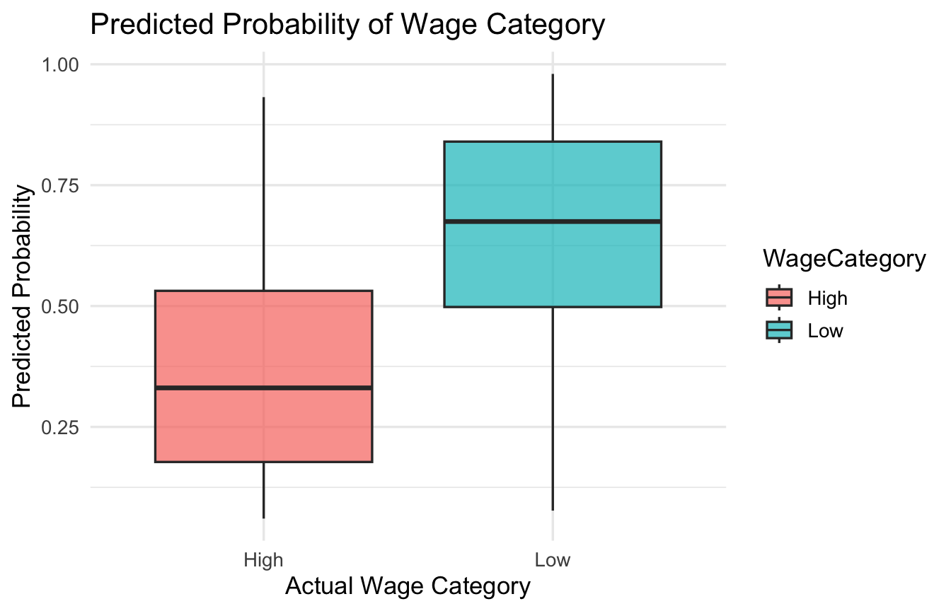
fig.cap = "A box plot representing the probability that two randomly chosen people will have their wages correctly predicted."Our AUC is 0.81 - this tells us that our model has very strong discriminative power and can accurately separate between high wage and low wages.
The model identifies high earners at a rate of 70%, and it identifies low earners at a rate of 75%. This model performs much better than the ‘No Information Rate’ performance, which is accurate about 51% of the time (0.72 > 0.51). So, this model is definitely better at predicting outcomes than guessing.
7.7 Step 6 – Final Interpretation
Based on all of the performed analyses, multiple variables were found to have a meaningful relationship with wage category. Specifically, a t-test showed a highly significant difference in the mean age of high earners (45 years) versus low earners (40 years). The ANOVA showed that education level is a statistically significant predictor of wages, accounting for 23% of the variance. Further, a chi-squared test indicated a statistically significant but weak association between race and wage category, suggesting that other factors likely play a larger role in determining wage category. The logistic regression model was made to predict wage category (Low vs. High) and identified multiple significant predictors. The summary(train_model) output suggested that age, marital status, education level, and health insurance status were the most impactful variables. Specifically, being older, having a college or advanced degree, being married, and having health insurance were all associated with a lower likelihood of earning a low wage. The strongest predictors of a high wage were having a college or advanced degree and having health insurance, as shown by the variable importance analysis. Evaluating the model’s performance had strong results. The model had an overall accuracy of 72% and a balanced accuracy of 72%, indicating it is effective at predicting wage category for both high and low earners. This model performs significantly better than the “No Information Rate,” which was approximately 51%. The model’s discriminative power was represented by a very high AUC (Area Under the Curve) of 0.81, which suggests the model can accurately distinguish between high and low wage earners 81% of the time. The Confusion Matrix also showed that the model performed slightly better at predicting low wage earners (sensitivity of 75%) than high wage earners (specificity of 70%). If this analysis were to be repeated, I would consider adding several new variables to potentially improve the model’s predictive power. Relevant additions could include a variable of specific job types or titles (instead of a broad jobclass), and location data, as different regions may result in different wages. Given the weak relationship found in the chi-squared test and the low variable importance, I would remove race from the model to make it more parsimonious. Ideally, these additions and removals would help to capture more of the complex factors that influence wage outcomes.