Chapter 2 Ch. 2: Conditional Probability
2.1 Theoretical Notes
2.1.1 Conditional probability.
Definition 2.2.1
If \(A\) and \(B\) are events with \(P(B)>0\), then the conditional probability of \(A\) given \(B\), is defined as \[ P(A\mid B) = \frac{P(A\cap B)}{P(B)}. \]
Pebble World intuition for \(P(A\mid B)\))
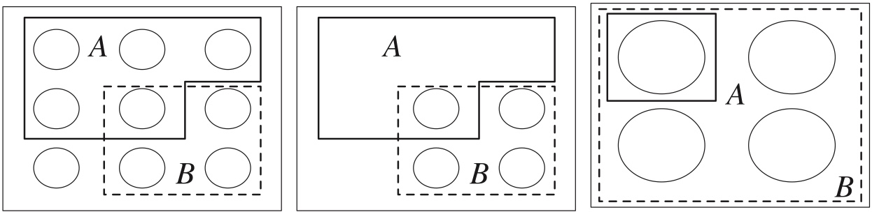
Figure 2.1: .
- Left: Events \(A\) and \(B\) are subsets of the sample space (total mass 1)
- Middle: We know that \(B\) occurred, so we get rid of \(B^c\)
- Right: In the restricted sample space, renormalize so the total mass is still 1
In the naïve definition of probability, a conditional probability is simply the probability evaluated over a sample space restricted by the conditioning event.
2.1.2 Bayes’ rule
Theorem 2.3.1
For any events \(A\) and \(B\) with positive probabilities, \[ P(A\cap B)=P(B)P(A\mid B)=P(A)P(B\mid A). \]
Theorem 2.3.2
For any events \(A_1,\ldots,A_n\) with positive probabilities, \[ \begin{split} P(A_1,A_2,\ldots,A_n) & = P(A_1)P(A_2\mid A_1)P(A_3\mid A_1,A_2)\cdots P(A_n\mid A_1,\ldots,A_{n-1}), \end{split} \] where the commas denote intersections.
Theorem 2.3.3 (Bayes’ rule) \[ P(A\mid B)=\frac{P(B\mid A)P(A)}{P(B)}. \] Bayes’ rule has important implications and applications in probability and statistics, since it is so often necessary to find conditional probabilities, and often \(P(B\mid A)\) is much easier to find directly than \(P(A\mid B)\) (or vice versa).
2.1.3 Odds
Definition 2.3.4
The odds of an event \(A\) are
\[ \mbox{odds}(A)=P(A)/P(A^c). \]
- For example, if \(P(A)=2/3\), we say the odds in favor of \(A\) are 2 to 1. (This is sometimes written as 2:1, and is sometimes stated as 1 to 2 odds against \(A\);
- care is needed since some sources do not explicitly state whether they are referring to odds in favor or odds against an event.
- We can also convert from odds back to probability:
\[ P(A)=\mbox{odds}(A)/(1+\mbox{odds}(A)). \]
Theorem 2.3.5 (Odds form of Bayes’ rule)
For any events \(A\) and \(B\) with positive probabilities, the odds of \(A\) after conditioning on \(B\) are
\[ \frac{P(A\mid B)}{P(A^c\mid B)}=\frac{P(B\mid A)}{P(B\mid A^c)}\frac{P(A)}{P(A^c)} \]
- In words, this says that the posterior odds \(P(A\mid B)/P(A^c\mid B)\) are equal to the prior odds \(P(A)/P(A^c)\) times the factor \(P(B\mid A)/P(B\mid A^c)\) , which is known in statistics as the likelihood ratio.
- Sometimes it is convenient to work with this form of Bayes’ rule to get the posterior odds, and then if desired we can convert from odds back to probability.
2.1.4 Law of total probability (LOTP).
Theorem 2.3.6
Let \(A_1,\ldots,A_n\) be a partition of the sample space \(S\) (i.e., the \(A_i\) are disjoint events and their union is \(S\)), with \(P(A_i)>0\) for all \(i\). Then \[ P(B)=\sum_{i=1}^n P(B\mid A_i)P(A_i) \]
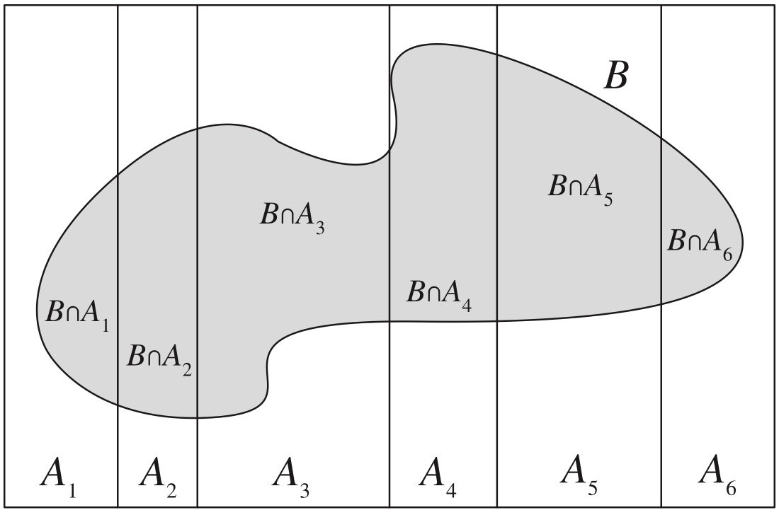
Figure 2.2: .
2.1.5 Conditional probabilities are probabilities
Any of the results about probability we have seen before are still valid if we condition on an event \(E\). In particular:
Conditional probabilities are between 0 and 1.
\(P(S\mid E)=1\), \(P(\emptyset\mid E)=0\).
If \(A_1,A_2,\ldots\) are disjoint, then \(P(\cup_{j=1}^\infty A_j\mid E)=\sum_{j=1}^\infty P(A_j\mid E)\).
\(P(A^c\mid E)=1-P(A\mid E)\).
Inclusion-exclusion: \(P(A\cup B \mid E)=P(A\mid E)+P(B\mid E)-P(A\cap B\mid E)\).
\(P(\cdot\mid E)\) assigns probabilities in accordance with the knowledge that \(E\) has occurred.
\(P(\cdot)\) is another probability function which assigns probabilities regardless of whether \(E\) has occurred or not.
Theorem 2.4.2 (Bayes’ rule with extra conditioning)
Provided that \(P(A\cap E)>0\) and \(P(B\cap E)>0\), we have \[ P(A\mid B,E)=\frac{P(B\mid A, E) P(A|E)}{P(B\mid E)}. \]
Recall: when we apply a condition, we restrain the sample space, while anything else remains the same.
Theorem 2.4.3 (LOTP with extra conditioning)
Let \(A_1,\ldots,A_n\) be a partition of \(S\). Provided that \(P(A_i\cap E)>0\) for all \(i\), we have \[ P(B\mid E)=\sum_{i=1}^n P(B\mid A_i,E)P(A_i\mid E). \]
2.1.6 Independence of events
Definition 2.5.1
Events \(A\) and \(B\) are independent if \[ P(A\cap B)=P(A)P(B). \] If \(P(A)>0\) and \(P(B)>0\), then this is equivalent to \(P(A\mid B)=P(A)\), and also equivalent to \(P(B\mid A)=P(B)\).
Independence is completely different from disjointness!
- If \(A\) and \(B\) are disjoint, then \(P(A\cap B)=0\), so disjoint events can be independent only if \(P(A)=0\) or \(P(B)=0\).
- Knowing that \(A\) occurs tells us that \(B\) definitely did not occur, so \(A\) clearly conveys information about \(B\), meaning the two events are not independent (except if \(A\) or \(B\) already has zero probability).
- Intuitively, it makes sense that if \(A\) provides no information about whether or not \(B\) occurred, then it also provides no information about whether or not \(B^c\) occurred.
Proposition 2.5.3
If \(A\) and \(B\) are independent, then \(A\) and \(B^c\) are independent, \(A^c\) and \(B\) are independent, and \(A^c\) and \(B^c\) are independent.
Definition 2.5.4 (Independence of three events)
Events \(A\), \(B\) and \(C\) are said to be independent if ALL the following equations hold:
\[ \begin{split} P(A\cap B) & = P(A)P(B) \\ P(A\cap C) & = P(A)P(C) \\ P(B\cap C) & = P(B)P(C) \\ \\ P(A\cap B \cap C) & = P(A)P(B)P(C). \end{split} \]
Example 2.5.5 (Pairwise independence doesn’t imply independence).
Consider two fair independent coin tosses, and let
\(A\) be the event that the first is Heads,
\(B\) the event that the second is Heads,
\(C\) the event that both tosses have the same result.
Then \(A\), \(B\), and \(C\) are pairwise independent but not independent, since \(P(A\cap B\cap C)=1/4\) while \(P(A)P(B) P(C)=1/8\).
The point is that just knowing about \(A\) or just knowing about \(B\) tells us nothing about \(C\), but knowing what happened with both \(A\) and \(B\) gives us information about \(C\) (in fact, in this case it gives us perfect information about \(C\)) .
On the other hand, \(P(A\cap B\cap C)=P(A)P(B) P(C)\) does not imply pairwise independence; this can be seen quickly by looking at the extreme case \(P(A)=0\) , when the equation becomes \(0=0\) , which tells us nothing about \(B\) and \(C\).
We can define independence of any number of events similarly.
Intuitively, the idea is that knowing what happened with any particular subset of the events gives us no information about what happened with the events not in that subset.
Definition 2.5.6 (Independence of many events).
For \(n\) events \(A_1, A_2,\ldots, A_n\) to be independent, we require any pair to satisfy \(P(A_i \cap A_j) = P(A_i)P(A_j)\) (for \(i\ne j\)), any triplet to satisfy \(P(A_i \cap A_j \cap A_k) = P(A_i)P(A_j)P(A_k)\) (for \(i\), \(j\), \(k\) distinct), and similarly for all quadruplets, quintuplets, and so on. For infinitely many events, we say that they are independent if every finite subset of the events is independent.
Definition 2.5.7 (Conditional independence).
Events \(A\) and \(B\) are said to be conditionally independent given \(E\) if \(P(A\cap B\mid E) = P(A\mid E)P(B\mid E)\).
2.5.8. It is easy to make terrible blunders stemming from confusing independence and conditional independence.
- Two events can be conditionally independent given \(E\), but not independent given \(E^c\).
- Two events can be conditionally independent given \(E\), but not independent.
- Two events can be independent, but not conditionally independent given \(E\).
- In particular, \(P(A,B)=P(A)P(B)\) does not imply \(P(A,B\mid E)=P(A\mid E)P(B\mid E)\); we can’t just insert “given E” everywhere, as we did in going from LOTP to LOTP with extra conditioning.
- This is because LOTP always holds (it is a consequence of the axioms of probability), whereas \(P (A,B)\) may or may not equal \(P(A)P(B)\), depending on what \(A\) and \(B\) are.
2.2 Examples
2.2.1 Example 2.2.2 (Two cards).
A standard deck of cards is shuffled well. Two cards are drawn randomly, one at a time without replacement. Let \(A\) be the event that the first card is a heart (\(\heartsuit\)), and \(B\) be the event that the second card is red (\(\heartsuit\), \(\diamondsuit\)). Find \(P(A\mid B)\) and \(P(B\mid A)\).
\[ P(A\mid B) = \frac{P(A\cap B)}{P(B)} \\ P(B\mid A) = \frac{P(A\cap B)}{P(A)} \] (topic: conditional probability, law of total probability)
solution:
First step is to find \(P(A\cap B)\).
The random experiment consists of two stages:
- Draw one card from a standard deck of \(52\) cards.
- Draw a second card from the remaining \(51\) cards.
The event \(A \cap B\) is defined as:
- Stage 1: the first card is a heart.
- Stage 2: the second card is red.
In Stage 1, there are \(52\) cards in total, of which \(13\) are hearts.
Thus,
\[
P(\text{heart on first draw}) = \frac{13}{52}.
\]
In Stage 2, only \(51\) cards remain. Since one heart (which is red) has already been taken, there are \(25\) red cards left.
Therefore,
\[
P(\text{red on second draw} \mid \text{heart on first draw}) = \frac{25}{51}.
\]
By the multiplication rule,
\[
P(A \cap B) = \frac{13}{52} \times \frac{25}{51}=\frac{25}{204}.
\]
The next step is to find \(P(A)\) and \(P(B)\).
The \(P(A)\) is simply \(1/4\) because there are \(13\) hearts among the \(52\) cards.
The calculation of \(P(B)\) is less straightforward. \[ P(B)=\frac{26}{52}\times \frac{51}{51}=\frac{1}{2} \]
since there are \(26\) favorable possibilities for the second card, and for each of those, the first card can be any other card (recall from Chapter 1 that chronological order is not needed in the multiplication rule).
If you find this not convincing enough, you can use the law of total probability (LOTP). Let’s define event \(C\) as obtaining a red card in the stage one, and \(C^c\) is its complement, then we have \[ P(B)=P(C\cap B)+P(C^c\cap B)=\frac{26}{52}\times \frac{25}{51}+\frac{26}{52}\times \frac{26}{51}=\frac{1}{2} \]
Finally, we have \[ P(A\mid B) = \frac{P(A\cap B)}{P(B)}=\frac{25/204}{1/2}=\frac{25}{102} \\ P(B\mid A) = \frac{P(A\cap B)}{P(A)}=\frac{25/204}{1/4}=\frac{25}{51} \] When we calculate conditional probability, the order matters! \[ P(A\mid B)\ne P(B\mid A) \]
2.2.2 Example 2.2.5 (Two children).
- A family has two children, and it is known that at least one is a girl.
- What is the probability that both are girls, given this information?
- What if it is known that the elder child is a girl?
The sample space is
- GB: 1st child is a girl, 2nd is a boy
- BG: 1st child is a boy, 2nd is a girl
- GG: both are girls
- BB: both are boys
Event \(A\): at least one is a girl
Event \(B\): both are girls, which is GG
Using the intuition of conditional probability, \(A\) reduced the sample space from four possible outcomes to three possible outcomes:
- GB
- BG
- GG
from which only one outcome (GG) favors event \(B\).
By the naive definition of probability, \(P(B\mid A)=\frac{1}{3}\).
If the condition becomes “the elder child is a girl”, the reduced sample space only contains GB and GG, thus, \(P(B\mid A)=\frac{1}{2}\).
2.2.3 Example 2.2.6 (Random child is a girl)
A family has two children. You randomly run into one of the two, and see that she is a girl. What is the probability that both are girls, given this information? Assume that you are equally likely to run into either child, and that which one you run into has nothing to do with gender.
This problem is less straight forward than the previous one, though they have the same story setting.
They key is how to interpret the information of “You randomly run into one of the two, and see that she is a girl.” Is it equivalent to “at least one child is a girl”? The answer is “No”!
This has sampling process involved. “You randomly run into one of the two, and see that she is a girl.” is equivalent to “you randomly sample a kid from the household and find the kid is a girl”. This cannot be easily computed by using naive definition of probability.
Let’s define events first.
\(A\): the random child is a girl
\(B\): both children are girls
We want to find out \[ P(B\mid A)=\frac{P(A \cap B)}{P(A)}. \]
We need to obtain \(P(A\cap B)\) and \(P(B)\).
The \(P(B)\) can be obtained using naive definition of probability, among \(4\) possible outcomes (GB, BG, GG, and BB), only one case (GG) favors the event \(B\), thus \[ P(B)=1/4 \]
Theorem 2.3.1 tells use that \[ P(A\cap B)=P(A \mid B)P(B). \] It is obvious that \(P(A\mid B)=P(\text{the random kid you see is a girl}\mid \text{both kids in the household are girls})=1\).
Thus , \[ P(A\cap B)=P(A \mid B)P(B)=1\times \frac{1}{4}=\frac{1}{4}. \] Now we need to find out \(P(A)\).
Is \(P(A)\) \(3/4\)? Of course not!
If the family has two boys, \(P(A)=0\); If the family has two girls, \(P(A)=1\); If the family has one boy and one girl, \(P(A)=1/2\).
We need to calculate \(P(A)\) by using LOTP.
Now partition the sample space into four, each partition contains one possible outcome.
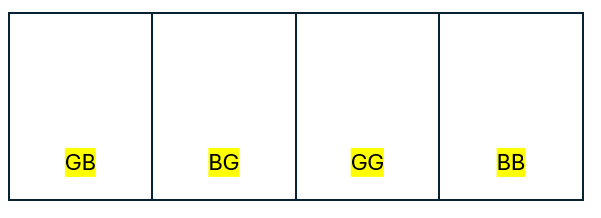
Figure 2.3: Partition of sample space for two children problem.
Denote partitions as \(C_1\) to \(C_4\)
\(C_1=GB\), \(C_2=BG\), \(C_3=GG\) and \(C_4=BB\).
By naive definition of probability, we know \(P(C_1)=P(C_2)=P(C_3)=P(C_4)=1/4\).
LOTP tells us that \[ \begin{split} P(A) &=P(A\cap C_1)+P(A\cap C_2)+P(A\cap C_3)+P(A\cap C_4) \\ &= P(A\mid C_1)P(C_1)+P(A\mid C_2)P(C_2)+P(A\mid C_3)P(C_3)+P(A\mid C_4)P(C_4) \end{split} \] If the family has two girls, you will ran into a girl for sure, so \(P(A\mid C_3)=1\)
If the family has two boys, there is no possibility to ran into a girl, so \(P(A\mid C_4)=0\).
If the family has one girl and one boy, the probability that you ran into a girl is \(1/2\), so \(P(A\mid C1)=P(A\mid C_2)=1/2\).
Thus, \[ \begin{split} P(A) &= P(A\mid C_1)P(C_1)+P(A\mid C_2)P(C_2)+P(A\mid C_3)P(C_3)+P(A\mid C_4)P(C_4) \\ &=1/2*1/4+1/2*1/4+1*1/4+0*1/4 \\ &=1/2 \end{split} \] Finally, we have \[ P(B\mid A)=\frac{P(A \cap B)}{P(A)}=\frac{1/4}{1/2}=1/2. \]
2.2.4 Example 2.2.7 (A girl born in winter).
A family has two children. Find the probability that both children are girls, given that at least one of the two is a girl who was born in winter. Assume that the four seasons are equally likely and that gender is independent of season (this means that knowing the gender gives no information about the probabilities of the seasons, and vice versa).
Event \(A\): at least one of the two is a girl born in winter
Event \(B\): both children are girls
Calculate \[ P(B\mid A)=\frac{P(A \cap B)}{P(A)} \] We go through the same steps in Example 2.2.6. \[ P(B\mid A)=\frac{P(A \cap B)}{P(A)}=\frac{P(A\mid B)P(B)}{P(A)} \] From previous examples, we already have \(P(B)=1/4\).
The calculation of \(P(A\mid B)\) is straightforward. If we know both kids are girls, the probability of having at least one girl born in winter is \[ P(A\mid B)= 1-P(\text{none of the two girls are born in winter})=1-\frac{3}{4}\times \frac{3}{4}=\frac{7}{16} \] The we have \[ P(A\cap B)=P(B)P(A\mid B)=\frac{1}{4}\times \frac{7}{16}=\frac{7}{64} \]
We use the same partition \(C_1\) to \(C_4\) in Figure 2.3 to calculate \(P(A)\) with LOTP.
If the family has one girl and one boy (in the case \(C_1\) and \(C_2\)), the probability that the girl was born in winter is \(1/4\). If the family has two girls, the probability that at least one of them was born in winter is \(1-3/4*3/4\). \[ \begin{split} P(A) &=P(A\mid C_1)P(C_1)+P(A\mid C_2)P(C_2)+P(A\mid C_3)P(C_3) \\ &=\frac{1}{4}\times \frac{1}{4}+\frac{1}{4}\times \frac{1}{4}+\frac{1}{4}\times \left(1-\frac{3}{4}\times\frac{3}{4}\right) \\ & =1/16+1/16+7/64=15/64 \end{split} \]
\[ P(B\mid A)=\frac{7/64}{15/64}=7/15 \]
2.2.5 Example 2.3.7 (Random coin).
You have one fair coin, and one biased coin which lands Heads with probability 3/4. You pick one of the coins at random and flip it three times. It lands Heads all three times. Given this information, what is the probability that the coin you picked is the fair one?
Define events:
\(A\): you picked the fair coin
\(B\): The coin gave you heads up all three times.
We need \(P(A \mid B)\), by Baye’s rule, \[ P(A \mid B)=\frac{P(B\mid A)P(A)}{P(B)}. \] We have \[ P(A)=\frac{1}{2} \]
\[ P(B\mid A)=P(\text{HHH}\mid \text{fair coin})=\left(\frac{1}{2}\right)^3 \]
\[ P(B\mid A^c)=P(\text{HHH}\mid \text{biased coin})=\left(\frac{3}{4}\right)^3 \]
By LOTP, \[ \begin{split} P(B)&=P(B\mid A)P(A)+P(B\mid A^c)P(A^c) \\ &= (1/8)*(1/2)+(27/64)*(1/2) \\ &=35/128 \end{split} \]
Thus, \[ P(A \mid B)=\frac{(1/8)*(1/2)}{35/128}\approx 0.23 \]
2.2.6 Example 2.3.9 (Testing for a rare disease).
A patient named Fred is tested for a disease called conditionitis, a medical condition that afflicts 1% of the population. The test result is positive, i.e., the test claims that Fred has the disease.
Let \(D\) be the event that Fred has the disease and \(T\) be the event that he tests positive. Suppose that the test is ``95% accurate’’; there are different measures of the accuracy of a test, but in this problem it is assumed to mean that \(P(T|D) = 0.95\) and \(P(T^c\mid D^c) = 0.95\).
The quantity \(P(T\mid D)\) is known as the sensitivity or true positive rate of the test, and \(P(T^c\mid D^c)\) is known as the specificity or true negative rate.
Find the conditional probability that Fred has conditionitis, given the evidence provided by the test result.
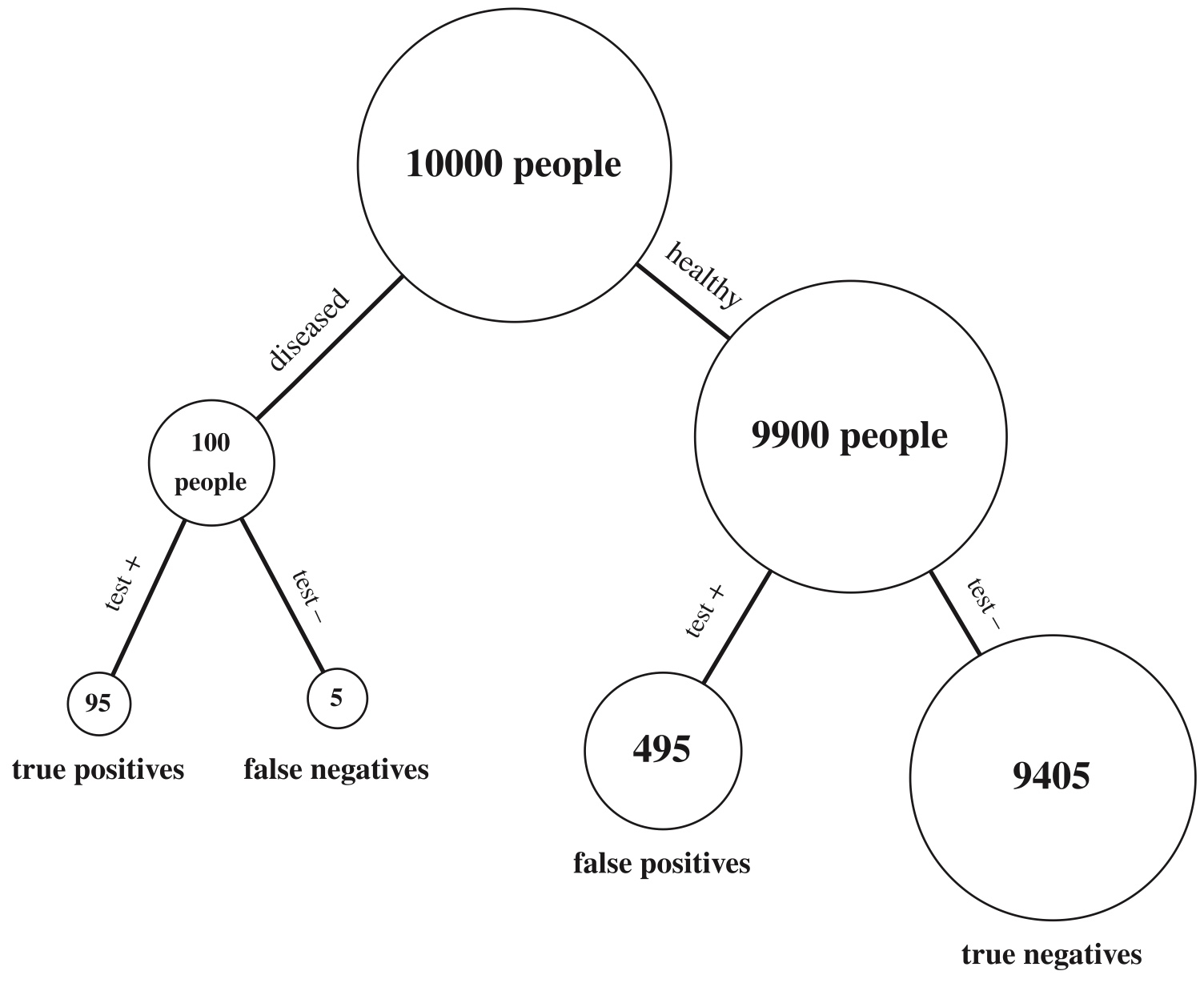
Figure 2.4: Testing for a rare disease.
We want to find \(P(D\mid T)\), and we know \[ P(D\mid T)=\frac{P(T\mid D)P(D)}{P(T)}. \] We already have \(P(T\mid D)=0.95\) and \(P(D)=1\%\).
By LOTP, \[ \begin{split} P(T)& = P(T|D)P(D)+P(T|D^c)P(D^c) \\ & =0.95*0.01 + (1-0.95)*0.99 \\ & = 0.059 \end{split} \] Thus, \[ P(D\mid T)=\frac{0.95*0.01}{0.059}=\frac{19}{118}=\approx 0.1610 \]
2.2.7 Example 2.3.10 (Six-fingered man).
A crime has been committed in a certain country. The perpetrator is one (and only one) of the \(n\) men who live in the country. Initially, these \(n\) men are all deemed equally likely to be the perpetrator. An eyewitness then reports that the crime was committed by a man with six fingers on his right hand.
Let \(p_0\) be the probability that an innocent man has six fingers on his right hand, and \(p_1\) be the probability that the perpetrator has six fingers on his right hand, with \(p_0<p_1\).
(We may have \(p_1<1\), since eyewitnesses are not 100% reliable.) Let \(a=p_0/p_1\) and \(b=(1-p_1)/(1-p_0)\). Rugen lives in the country. He is found to have six fingers on his right hand.
Given this information, what is the probability that Rugen is the perpetrator?
If we pick a random man from that country, Define event \(A\) as that man has six fingers, and event \(B\) as that man is the perpetrator.
The information tells us that
- \(P(A \mid B^c)=p_0\), given that the man is innocent, the probability that he has six fingers is \(p_0\);
- \(P(A\mid B)=p_1\), given that the man is guilty, the probability that he has six fingers is \(p_1\);
- \(P(B)=1/n\), overall, the probability that a random man has six fingers is \(1/n\).
By Bayes’ Rule \[ P(B\mid A)=\frac{P(A\cap B)}{P(A)}=\frac{P(A\mid B)P(B)}{P(A)}=\frac{p_1/n}{P(A)} \] By LOTP, \[ \begin{split} P(A)& =P(A\mid B^c)P(B^c)+P(A\mid B)P(B)\\ &=p_0\times \left (1-\frac{1}{n}\right )+p_1\times \frac{1}{n} \\ &=p_0-\frac{p_0-p_1}{n} \end{split} \] Thus, \[ P(B\mid A)=\frac{p_1/n}{P(A)}=\frac{p_1/n}{p_0-\frac{p_0-p_1}{n}}=\frac{1}{np_0/p_1-p_0/p_1+1}=\frac{1}{na-a+1} \]
Now suppose that all \(n\) men who live in the country have their hands checked, and Rugen is the only one with six fingers on his right hand. Given this information, what is the probability that Rugen is the perpetrator?
Now we have extra information, which is “all other men except the picked one do not have six fingers”,
so we can append this information as an extra condition on the Bayes’ rule
\[ P(B\mid A, C)=\frac{P(A, C\mid B)P(B)}{P(A, C)}=\frac{P(A\mid B, C)P(B\mid C)}{P(A\mid C)} \]
where \(C\) is “all other men do not have with fingers on their right hands”. $$
$$
\[ P(A, C \mid B)=P(\text{the random man has six fingers and all other men do not have six fingers}\mid \text{the man is guilty}) \]
\[ P(A\cap C \mid B)= P(A\mid B)P(C\mid A, B) \]
We already have \(P(A\mid B)=p_1\) and \(P(B)=1/n\).
The probability \(P(C \mid A, B)\) can be interpreted as “Given that one man is guilty and he has six fingers, what is the probability that all other innocent men have five fingers on their right hand”. \[ P(C \mid A, B)=(1-p_0)^{n-1} \] \[ P(A, C \mid B)=p_1(1-p_0)^{n-1} \]
The next step is to computer \(P(A ,C)\) using LOTP. \[ P(A, C)=P(A, C\mid B)P(B)+P(A, C\mid B^c)P(B^c) \]
We already have the first term, only need the second one. \[ P(A, C \mid B^c)=p_0(1-p_1)(1-p_0)^{n-2} \]
We can interpreted \(p_0(1-p_1)(1-p_0)^{n-2}\) as the conditional probability of “Rugen has 6 fingers” AND “the perpetrator has 6 fingers” AND “non of the rest n-2 people have six fingers”.
\[ P(A, C)=P(A, C\mid B)P(B)+P(A, C\mid B^c)P(B^c)=p_1(1-p_0)^{n-1}(1/n)+p_0(1-p_1)(1-p_0)^{n-2}(1-1/n) \]
Thus, \[ P(B\mid A, C)=\frac{P(A, C\mid B)P(B)}{P(A, C)}=\frac{p_1(1-p_0)^{n-1}(1/n)}{p_1(1-p_0)^{n-1}(1/n)+p_0(1-p_1)(1-p_0)^{n-2}(1-1/n)} \]
2.2.8 Example 2.4.4 (Random coin, continued).
You have one fair coin, and one biased coin which lands Heads with probability 3/4. You pick one of the coins at random and flip it three times.
Suppose we have now seen our chosen coin land Heads three times. If we toss the coin a fourth time, what is the probability that it will land Heads once more?
Define events:
- \(A\): picked the fair coin
- \(B\): landed Heads three times
- \(C\): land Head at the \(4\)th time
Information we have:
- \(P(A)=1/2\) and \(P(A^c)=1/2\)
- \(P(B\mid A)=(1/2)^3=1/8\)
- \(P(B\mid A^c)= (3/4)^3\)
From Example 2.3.7, we already have \[ \begin{split} P(B)&=P(B\mid A)P(A)+P(B\mid A^c)P(A^c) \\ &= (1/8)*(1/2)+(27/64)*(1/2) \\ &=35/128 \end{split} \] and \[ P(A \mid B)=\frac{(1/8)*(1/2)}{35/128}=8/35\approx 0.23 \] Of course, \[ P(A^c\mid B) \approx 1-0.23=0.77 \] We want to find the probability of \(P(C \mid B)\)
By LOTP with extra condition (which is B), \[ P(C\mid B) =P(C \mid A, B)P(A\mid B)+P(C \mid A^c, B)P(A^c\mid B) \]
\[ P(C\mid A, B)=P(C\mid A)=1/2 \]
\[ P(C\mid A^c, B)=P(C\mid A^c)=3/4 \]
Event \(A\) has all the information given by \(B\), this is why \(P(C\mid A, B)=P(C\mid A)\). In other words, given \(A\), \(B\) and \(C\) are independent.
Thus, \[ \begin{split} P(C\mid B) & =P(C \mid A, B)P(A\mid B)+P(C \mid A^c, B)P(A^c\mid B) \\ &= 1/2*8/35+3/4*27/35 \\ &= 97/140 \approx 0.693 \end{split} \]
2.2.9 Example 2.4.5 (Unanimous agreement).
The article “Why too much evidence can be a bad thing”” by Lisa Zyga says:
Under ancient Jewish law, if a suspect on trial was unanimously found guilty by all judges, then the suspect was acquitted. This reasoning sounds counterintuitive, but the legislators of the time had noticed that unanimous agreement often indicates the presence of systemic error in the judicial process.
There are \(n\) judges deciding a case. The suspect has prior probability \(p\) of being guilty. Each judge votes whether to convict or acquit the suspect. With probability \(s\), a systemic error occurs (e.g., the defense is incompetent). If a systemic error occurs, then the judges unanimously vote to convict (i.e., all \(n\) judges vote to convict). Whether a systemic error occurs is independent of whether the suspect is guilty.
Given that a systemic error doesn’t occur and that the suspect is guilty, each judge has probability \(c\) of voting to convict, independently. Given that a systemic error doesn’t occur and that the suspect is not guilty, each judge has probability \(w\) of voting to convict, independently. Suppose that \[ 0<p<1, 0<s<1, \;\;\mbox{and}\;\; 0<w<\frac{1}{2}<c<1. \]
First step is to define events:
- \(A\): the suspect is guilty
- \(S\): a systemic error occur
- \(A\) and \(S\) are independent!
We have:
\(P(A)=p\)
\(P(S)=s\)
Besides, \[ P(\text{a judge vote to convict}\mid A, S^c)=c \]
\[ P(\text{a judge vote to convict}\mid A^c, S^c)=w \]
- For this part only, suppose that exactly \(k\) out of \(n\) judges vote to convict, where \(k<n\). Given this information, find the probability that the suspect is guilty.
Be ware that the systemic error did not occur.
Define another event \(C\): exact \(k\) judges vote to convict
We want to find \(P(A\mid C, S^c)\). \[ P(A\mid C, S^c)=\frac{P(C\mid A, S^c)P(A\mid S^c)}{P(C\mid S^c)} \]
\[ P(C\mid A, S^c)=c^k(1-c)^{n-k} \]
\(A\) and \(S\) are independent, so \(P(A\mid S^c)=P(A)=p\).
Similarly, we have \[ P(C\mid A^c, S^c)=w^k(1-w)^{n-k} \] By LOTP with extra conditions, \[ P(C\mid S^c)=P(C\mid A, S^c)P(A\mid S^c)+P(C\mid A^c, S^c)P(A^c\mid S^c)=pc^k(1-c)^{n-k}+(1-p)w^k(1-w)^{n-k} \]
Finally, we have \[ P(A\mid C, S^c)=\frac{P(C\mid A, S^c)P(A\mid S^c)}{P(C\mid S^c)}=\frac{pc^k(1-c)^{n-k}}{pc^k(1-c)^{n-k}+(1-p)w^k(1-w)^{n-k}} \]
- Now suppose that all \(n\) judges vote to convict. Given this information, find the probability that the suspect is guilty.
This time, we cannot tell if the systemic error occurs or not.
Define event \(D\): all \(n\) judges vote to convict
We want \(P(A\mid D)\). \[ P(A\mid D)= \frac{P(D\mid A)P(A)}{P(D)} \]
\[ P(D\mid A)=P(D\mid S, A)P(S\mid A)+P(D\mid S^c, A)P(S^c\mid A)=s+c^n(1-s) \]
\[ P(D)=P(D\mid A)P(A)+P(D\mid A^c)P(A^c) \]
\[ P(D\mid A^c)=P(D\mid S,A^c)P( S\mid A^c)+P(D\mid S^c, A^c)P(S^c\mid A^c)=s+w^n(1-s) \]
Eventually, we have \[ P(A\mid D)= \frac{P(D\mid A)P(A)}{P(D)}=\frac{p(s+c^n(1-s))}{p(s+c^n(1-s))+(1-p)(s+w^n(1-s))} \]
- Is the answer to (b), viewed as a function of \(n\), an increasing function?
By calculus, it is easy to see that \[ \lim_{n\rightarrow n} P(A\mid D) =p \]
2.2.10 Example 2.5.9 (Conditional independence doesn’t imply independence).
Returning once more to the scenario from Example 2.3.7, suppose we have chosen either a fair coin or a biased coin with probability \(\frac{3}{4}\) of heads, but we do not know which one we have chosen. We flip the coin a number of times. Conditional on choosing the fair coin, the coin tosses are independent, with each toss having probability \(\frac{1}{2}\) of heads. Similarly, conditional on choosing the biased coin, the tosses are independent, each with probability \(\frac{3}{4}\) of heads.
2.2.11 Example 2.5.10 (Independence doesn’t imply conditional independence).
Suppose that my friends Alice and Bob are the only two people who ever call me. Each day, they decide independently whether to call me: letting \(A\) be the event that Alice calls and \(B\) be the event that Bob calls, A and B are unconditionally independent. But suppose that I hear the phone ringing now. Conditional on this observation, \(A\) and \(B\) are no longer independent: if the phone call isn’t from Alice, it must be from Bob. In other words, letting \(R\) be the event that the phone is ringing, we have \(P(B\mid R) < 1 = P(B\mid A^c, R)\), so \(B\) and \(A^c\) are not conditionally independent given \(R\), and likewise for \(A\) and \(B\).
2.2.12 Example 2.5.11 (Conditional independence given \(E\) vs. given \(E^c\)).
Suppose there are two types of classes: good classes and bad classes. In good classes, if you work hard, you are very likely to get an \(A\). In bad classes, the professor randomly assigns grades to students regardless of their effort. Let \(G\) be the event that a class is good, \(W\) be the event that you work hard, and \(A\) be the event that you receive an A. Then \(W\) and \(A\) are conditionally independent given \(G^c\), but they are not conditionally independent given \(G\)!
2.2.13 Example 2.5.12. (Why is the baby crying?)
A certain baby cries if and only if she is hungry, tired, or both. Let \(C\) be the event that the baby is crying, \(H\) be the event that she is hungry, and \(T\) be the event that she is tired. Let \(P(C)=c\), \(P(H)=h\), and \(P(T)=t\), where none of \(c\), \(h\) or \(t\) are equal to \(0\) or \(1\). Let \(H\) and \(T\) be independent.
Events:
- \(C\) be the event that the baby is crying,
- \(H\) be the event that she is hungry,
- \(T\) be the event that she is tired.
and
- $ P(C)=c$,
- \(P(H)=h\),
- \(P(T)=t\),
- Find \(c\), in terms of \(h\) and \(t\).
\[ c=P(C)=P(H \cup T)=P(H)+P(T)-P(H\cap T)=h+t-ht \]
- Find \(P(H\mid C)\), \(P(T\mid C)\) and \(P(H,T\mid C)\). \[ P(H\mid C)=\frac{P(C\mid H)P(H)}{P(C)}=\frac{1*h}{c}=h/c \] similarly, we have \[ P(T\mid C)=t/c \]
\[ P(H, T\mid C)=\frac{P(C\mid H, T)P(H, T)}{P(C)}=\frac{1*ht}{c}=ht/c \] Recall: \(H,T=H\cap T\), which IS a joint event. If we denote \(D=H\cap T\), the formula is very straightforward \[ P(H, T\mid C)=P(D\mid C)=\frac{P(C\mid D)P(D)}{P(C)} \] (c) Are \(H\) and \(T\) conditionally independent given \(C\)? Explain in two ways: algebraically using the quantities from (b), and with an intuitive explanation in words. \[ P(H, T\mid C)=\frac{ht}{c}\ne P(H\mid C)P(T\mid C)=\frac{ht}{c^2} \] so \(H\) and \(T\) are not conditionally independent.
Intuitively, if the bay is crying but not hungry, he must be tired.
2.2.14 Example 2.6.1 (Testing for a rare disease, continued).
Fred, who tested positive for conditionitis in Example 2.3.9, decides to get tested a second time. The new test is independent of the original test (given his disease status) and has the same sensitivity and specificity. Unfortunately for Fred, he tests positive a second time. Find the probability that Fred has the disease, given the evidence, in two ways:
- in one step, conditioning on both test results simultaneously, and
- in two steps, first updating the probabilities based on the first test result, and then updating again based on the second test result.
Recall: Let \(D\) be the event that Fred has the disease and \(T\) be the event that he tests positive. Suppose that the test is ``95% accurate’’; there are different measures of the accuracy of a test, but in this problem it is assumed to mean that \(P(T|D) = 0.95\) and \(P(T^c\mid D^c) = 0.95\). \(P(D)=0.01\)
Define
- \(T_1\): as test positive in the first test
- \(T_2\): as test positive in the 2nd test
One step method: \[ P(D\mid T_1, T_2)=\frac{P(T_1, T_2\mid D)P(D)}{P(T1, T_2)} \]
\[ P(T_1, T_2\mid D)=P(T_1\mid D)P(T_2\mid D)=0.95^2 \]
\[ P(T_1, T_2)=P(T_1,T_2 \mid D)P(D)+P(T_1, T_2\mid D^c)P(D^c)=0.95^2*0.01+0.05^2*0.99 \]
Thus, \[ P(D\mid T_1, T_2)=\frac{P(T_1, T_2\mid D)P(D)}{P(T1, T_2)}=\frac{0.95^2*0.01}{0.95^2*0.01+0.05^2*0.99}\approx 0.78 \] Two steps method: \[ P(D\mid T_1) =0.1610 \]
\[ P(D\mid T_1, T_2)=\frac{P(T_2 \mid D, T_1)P(D\mid T_1)}{P(T_2\mid T_1)} \]
\[ P(T_2 \mid D, T_1)=P(T_2\mid T_1, D)=P(T_2\mid D)=0.95 \]
\[ P(T_2\mid T_1)=P(T_2\mid D, T_1)P(D\mid T_1)+P(T_2\mid D^c, T_1)P(D^c\mid T_1)=0.95*(0.1610)+0.05*(1-0.1610) \]
Finally, we have \[ P(D\mid T_1, T_2)=\frac{P(T_2 \mid D, T_1)P(D\mid T_1)}{P(T_2\mid T_1)}=\frac{0.95*0.1610}{0.95*0.1610+0.05*(1-0.1610)}\approx 0.78 \]
2.2.15 Example 2.7.1 (Monty Hall).
On the game show Let’s Make a Deal, hosted by Monty Hall, a contestant chooses one of three closed doors, two of which have a goat behind them and one of which has a car. Monty, who knows where the car is, then opens one of the two remaining doors. The door he opens always has a goat behind it (he never reveals the car!). If he has a choice, then he picks a door at random with equal probabilities. Monty then offers the contestant the option of switching to the other unopened door. If the contestant’s goal is to get the car, should she switch doors?
http://www.rossmanchance.com/applets/MontyHall/Monty04.html
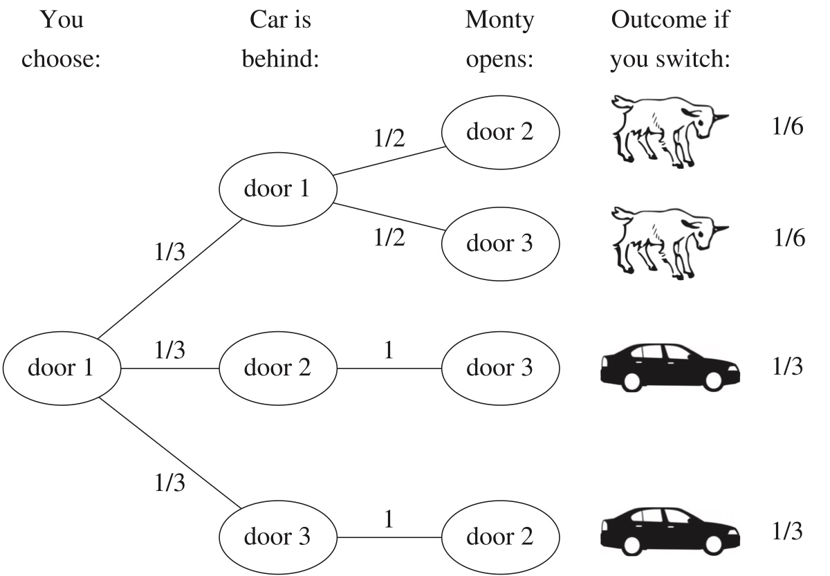
Figure 2.5: .
A typical use of conditional probabilities is to make the calculation easier. In many cases, the conditional probability is much easier to compute than the unconditional one.
Suppose the contestant picked door \(1\), which has a car behind of it.
Define \(C_i\) as the car is behind door \(i\), \(i=1, 2, 3\).
\(P(C_i)=1/3\).
We use \(C_i\)s as conditions to calculate the probability of getting a car.
By LOTP, \[ P(\text{get a car})=P(\text{get a car}\mid C_1)P(C_1)+P(\text{get a car}\mid C_2)P(C_2)+P(\text{get a car}\mid C_3)P(C_3) \] Suppose the contestant uses the switching strategy: \[ P(\text{get a car}\mid C_1)=0 \]
\[ P(\text{get a car}\mid C_2)=1 \]
\[ P(\text{get a car}\mid C_3)=1 \]
Thus, if use switching strategy, \[ P(\text{get a car})=0*1/3+1*1/3+1*1/3=2/3 \]
When the contestant chooses whether to switch, she also knows which door Monty opened. We showed that the unconditional probability of success is \(2/3\) (when following the switching strategy), but let’s also show that the conditional probability of success for switching, given the information that Monty provides, is also \(2/3\).
Let \(M_j\) be the event that Monty opens door \(j\), for \(j = 2,3\). Then
\[ P(\text{get car}) = P(\text{get car} \mid M_2)P(M_2) + P(\text{get car} \mid M_3)P(M_3), \]
where by symmetry \(P(M_2) = P(M_3) = 1/2\) and \(P(\text{get car}\mid M_2) = P(\text{get car}\mid M_3)\).
Let
\[ x = P(\text{get car} \mid M_2) = P(\text{get car} \mid M_3). \]
Plugging in what we know,
\[ \frac{2}{3} = P(\text{get car}) = \frac{x}{2} + \frac{x}{2} = x, \]
as claimed.
Bayes’ rule also works nicely for finding the conditional probability of success using the switching strategy, given the evidence. Suppose that Monty opens door 2. Using the notation and results above,
\[ P(C_1 \mid M_2) = \frac{P(M_2 \mid C_1) P(C_1)}{P(M_2)} = \frac{(1/2)(1/3)}{1/2} = \frac{1}{3}. \]
So given that Monty opens door 2, there is a \(1/3\) chance that the contestant’s original choice of door has the car, which means that there is a \(2/3\) chance that the switching strategy will succeed.
Exercise 41.
After the contestant chooses a door, Monty flips a coin with \(P(H)=p\). If it lands Head up, then Monty opens a door with goat (just like the original question). If the coin lands tail up, then Monty opens one of remaining doors (no matter what is behind of it).
Now, suppose it turned out that the contestant chooses door 1 and the then Monty opens door 2. What is the probability of success if they switch to door 3?
Solution:
For \(j = 1,2,3\), let \(C_j\) be the event that the car is behind door \(j\),
\(G_j = C_j^c\), and \(M_j\) be the event that Monty opens door \(j\).
We want to find out \[ P(C_3 \mid M_2, G_2) \] Let \(R\) be the event that Monty is in “random mode” (i.e., the coin lands Tails).
If Monty is not in random mode (coin lands head up), we already have \[ P(C_3 \mid M_2, G_2, R^c)=2/3 \] By the law of total probability, \[ P(C_3 \mid M_2, G_2) = P(R \mid M_2, G_2) P(C_3 \mid M_2, G_2, R) + P(R^c \mid M_2, G_2) P(C_3 \mid M_2, G_2, R^c), \]
where
\[ P(C_3 \mid M_2, G_2, R^c) = \tfrac{2}{3} \quad \text{(since given $R^c$, Monty is operating as in the usual Monty Hall problem)} \]
and
\[ P(C_3 \mid M_2, G_2, R) = \frac{P(M_2, G_2 \mid C_3, R) P(C_3 \mid R)}{P(M_2, G_2 \mid R)} = \frac{\tfrac{1}{2} \cdot \tfrac{1}{3}}{\tfrac{1}{2} \cdot \tfrac{2}{3}} = \tfrac{1}{2}. \]
For the denominator above, note that \(M_2\) and \(G_2\) are conditionally independent given \(R\);
for the numerator, note also that \(P(M_2, G_2 \mid C_3, R) = P(M_2 \mid C_3, R) = P(M_2 \mid R)\).
The posterior probability that Monty is in random mode is
\[ P(R \mid M_2, G_2) = \frac{P(M_2, G_2 \mid R) P(R)}{P(M_2, G_2 \mid R) P(R) + P(M_2, G_2 \mid R^c) P(R^c)} = \frac{\tfrac{1}{2} \cdot \tfrac{2}{3} (1-p)}{\tfrac{1}{2} \cdot \tfrac{2}{3} (1-p) + \tfrac{1}{2} p} = \frac{2(1-p)}{2+p}, \]
again since \(M_2\) and \(G_2\) are conditionally independent given \(R\), and since given \(R^c\), \(M_2\) implies \(G_2\).
Putting these results together, we have
\[ P(C_3 \mid M_2, G_2) = \tfrac{1}{2} \cdot \frac{2(1-p)}{2+p} + \tfrac{2}{3} \left( 1 - \frac{2(1-p)}{2+p} \right) = \frac{1+p}{2+p}. \]
2.2.16 Example 2.7.2 (Branching process).
A single amoeba, Bobo, lives in a pond. After one minute Bobo will either die, split into two amoebas, or stay the same, with equal probability, and in subsequent minutes all living amoebas will behave the same way, independently. What is the probability that the amoeba population will eventually die out?
Define events:
- \(D\): the population eventually dies out;
- \(B_i\): Bobo turns into \(i\) amoebas, \(i=0, 1, 2\).
\[ P(D \mid B_0)=1 \]
\[ P(D\mid B_1)=P(D) \]
\[ P(D\mid B_2)=[P(D)]^2 \]
By LOTP, \[ \begin{split} P(D)&=P(D \mid B_0)P(B_0)+P(D \mid B_1P(B_1)+P(D \mid B_2)P(B_2) \\ &=1*1/3+P(D)*1/3+[P(D)]^2*1/3 \end{split} \] Solving the equation, we will get \[ P(D)=1 \]
2.2.17 Example 2.7.3 (Gambler’s ruin).
Two gamblers, A and B, make a sequence of $1 bets. In each bet, gambler A has probability \(p\) of winning, and gambler B has probability \(q=1-p\) of winning. Gambler A starts with \(i\) dollars and gambler B starts with \(N-i\) dollars; the total wealth between the two remains constant since every time A loses a dollar, the dollar goes to B, and vice versa.
We can visualize this game as a random walk on the integers between 0 and \(N\), where \(p\) is the probability of going to the right in a given step: imagine a person who starts at position \(i\) and at each time step moves one step to the right with probability \(p\) and one step to the left with probability \(q=1-p\). The game ends when either A or B is ruined, i.e., when the random walk reaches 0 or \(N\). What is the probability that A wins the game (walking away with all the money)?
Let \(R_n\) the total fortune after the \(n\)th gamble.
\(R_n=\Delta_1+\ldots +\Delta_n\), \(R_0=i\), where \(P(\Delta=1)=p\) and \(P(\Delta=-1)=q\).
The game stops when either \(R_n=0\) or \(R_n=N\).
Let \(\tau_i=\min\{n\geq 0: R_n\in\{0,N\}\mid R_0=i\}\) denote the time at which the game stops when \(R_0=i\).
If \(R_{\tau_i}=N\), then the gambler wins; if \(R_{\tau_i}=0\), then the gambler is ruined.
Let \(P_i=P(R_{\tau_i}=N)\) denote the probability that the gambler wins when \(R_0=i\).
- \(P_0=0\) and \(P_N=1\).
We need to find \(P_i\), \(1\leq i\leq N-1\). We will condition on the outcome of the first gamble, \(\Delta_1=1\) or \(\Delta_1=-1\).
If \(\Delta_1=1\), then the gambler’s total fortune increases to \(R_1=i+1\), so the gambler will now win with probability \(P_{i+1}\).
Similarly, if \(\Delta_1=-1\), then the gambler’s fortune decreases to \(R_1=i-1\), so the gambler will now win with proability \(P_{i-1}\).
The probabilities corresponding to these two outcomes are \(p\) and \(q\), respectively, leading to \[ P_i=p P_{i+1}+ q P_{i-1}. \]
This is a difference equation with a characteristic polynomial \[ px^2-x+q=0 \] whose roots are 1 and \(\frac{q}{p}\).
If \(p\ne 1/2\) these roots are distinct with a general solution \[ P_i= a \cdot 1^i +b\cdot\Bigl(\frac{q}{p}\Bigr)^i. \]
- Using the boundary conditions \(P_0=0\) and \(P_N=1\), \[ a=-b=\frac{1}{1-\Bigl(\frac{q}{p}\Bigr)^N}. \]
- If \(p=1/2\), the root of the characteristic polynomial is equal to 1 and the general solution is \[ P_i= a \cdot 1^i +b\cdot i\cdot 1^i \] and from the boundary conditions it follows that \(a=0\) and \(b=\frac{1}{N}\), so \[ P_i=\left\{ \begin{array}{ll} \frac{1-\Bigl(\frac{q}{p}\Bigr)^i}{1-\Bigl(\frac{q}{p}\Bigr)^{N}} & \mbox{if}\;\; p\ne 1/2\\ \frac{i}{N} & \mbox{if}\;\; p=1/2. \end{array} \right. \]
2.2.19 Biohazard 2.8.1 (Prosecutor’s fallacy).
In 1998, Sally Clark was tried for murder after two of her sons died shortly after birth. During the trial, an expert witness for the prosecution testified that the probability of a newborn dying of sudden infant death syndrome (SIDS) was 1/8500, so the probability of two deaths due to SIDS in one family was \((1/8500)^2\), or about one in 73 million. Therefore, he continued, the probability of Clark’s innocence was one in 73 million.
- There are at least two major problems with this line of reasoning.
- First, the expert witness found the probability of the intersection of “first son dies of SIDS” and “second son dies of SIDS” by multiplying the individual event probabilities; as we know, this is only valid if deaths due to SIDS are independent within a family.
- Second, the so-called expert has confused two different conditional probabilities: \(P(\mbox{innocence}\mid \mbox{evidence})\) is different from \(P(\mbox{evidence}\mid \mbox{innocence})\). The witness claims that the probability of observing two newborn deaths if the defendant were innocent is extremely low; that is, \(P(\mbox{evidence}\mid \mbox{innocence})\) is small. What we are interested in, however, is \(P(\mbox{innocence}\mid \mbox{evidence})\), the probability that the defendant is innocent given all the evidence. By Bayes’ rule,
\[ P(\mbox{innocence}\mid \mbox{evidence})=\frac{P(\mbox{evidence}\mid \mbox{innocence})P(\mbox{Innocence})}{P(\mbox{evidence})}. \]
So to calculate the conditional probability of innocence given the evidence, we must take into account \(P(\mbox{innocence})\), the prior probability of innocence. This probability is extremely high: although double deaths due to SIDS are rare, so are double infanticides! The posterior probability of innocence given the evidence is a balance between P(evidence|innocence), which is low, and P(innocence), which is high.
2.2.20 Example 2.8.2 (Defense attorney’s fallacy).
A woman has been murdered, and her husband is put on trial for this crime. Evidence comes to light that the defendant had a history of abusing his wife. The defense attorney argues that the evidence of abuse should be excluded on grounds of irrelevance, since only 1 in 10,000 men who abuse their wives subsequently murder them. Should the judge grant the defense attorney’s motion to bar this evidence from trial?
Suppose that the defense attorney’s 1-in-10,000 figure is correct, and further assume the following facts:
- 1 in 10 men commit abuse against their wives.
- 1 in 5 married women who are murdered are murdered by their husbands.
- 50% of husbands who murder their wives previously abused them.
Let
- \(A\) be the event that the husband commits abuse against his wife.
- \(G\) be the event that the husband is guilty. The defense’s argument is that \(P(G\mid A) = 1/10,000\), so guilt is still extremely unlikely conditional on a previous history of abuse.
However, the defense attorney fails to condition on a crucial fact: in this case, we know that the wife was murdered. Therefore, the relevant probability is not \(P(G\mid A)\), but \(P(G\mid A, M)\), where \(M\) is the event that the wife was murdered.
Bayes’ rule with extra conditioning gives \[ \begin{split} P(G\mid A,M) & = \frac{P(A\mid G,M)P(G\mid M)}{P(A\mid G,M)P(G\mid M)+P(A\mid G^c,M)P(G^c\mid M)} \\ & = \frac{(.5)(.2)}{(.5)(.2)+(.1)(.8)} \\ & = \frac{5}{9}. \end{split} \]
\(P(G\mid A)\) was not used in the calculation, because it does not account for the fact that the wife was murdered.
2.2.21 Example 2.8.3 (Simpson’s paradox).
Two doctors, Dr. Hibbert and Dr. Nick, each perform two types of surgeries: heart surgery and Band-Aid removal. Each surgery can be either a success or a failure. The two doctors’ respective records are given in the following tables, and shown graphically in Figure 2.6, where white dots represent successful surgeries and black dots represent failed surgeries.
Dr. Hibbert
| Heart | Band-Aid | |
|---|---|---|
| Success | 70 | 10 |
| Failure | 20 | 0 |
Dr. Nick
| Heart | Band-Aid | |
|---|---|---|
| Success | 2 | 81 |
| Failure | 8 | 9 |
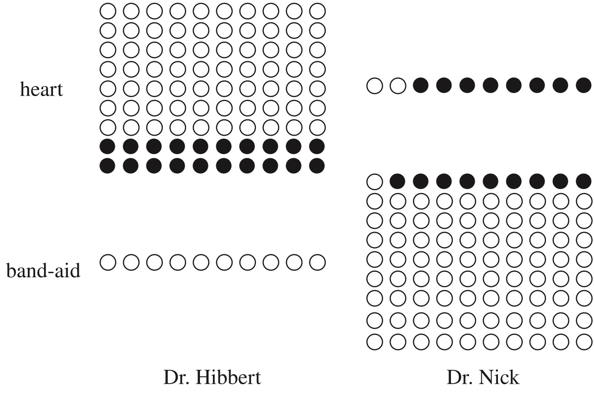
Figure 2.6: .
- Dr. Hibbert had a higher success rate than Dr. Nick in heart surgeries: 70 out of 90 versus 2 out of 10.
- Dr. Hibbert also had a higher success rate in Band-Aid removal: 10 out of 10 versus 81 out of 90.
- But if we aggregate across the two types of surgeries to compare overall surgery success rates, Dr. Hibbert was successful in 80 out of 100 surgeries while Dr. Nick was successful in 83 out of 100 surgeries: Dr. Nick’s overall success rate is higher!
- What’s happening is that Dr. Hibbert, presumably due to his reputation as the superior doctor, is performing a greater number of heart surgeries, which are inherently riskier than Band-Aid removals. His overall success rate is lower not because of lesser skill on any particular type of surgery, but because a larger fraction of his surgeries are risky.
2.2.22 Simpson’s paradox
For events \(A\), \(B\) and \(C\), we say that we have a Simpson’s paradox if \[ \begin{split} P(A\mid B,C) & < P(A\mid B^c, C) \\ P(A\mid B,C^c) & < P(A\mid B^c, C^c) \end{split} \] but \[ P(A\mid B) > P(A\mid B^c). \]
- In this case, let
- \(A\) be the event of a successful surgery.
- \(B\) be the event that Dr. Nick is the surgeon.
- \(C\) be the event that the surgery is a heart surgery.
- The conditions for Simpson’s paradox are fulfilled because the probability of a successful surgery is lower under Dr. Nick than under Dr. Hibbert whether we condition on heart surgery or on Band-Aid removal, but the overall probability of success is higher for Dr. Nick.
The law of total probability tells us mathematically why this can happen: \[ \begin{split} P(A\mid B) & = P(A\mid C,B)P(C\mid B)+P(A\mid C^c,B)P(C^c\mid B) \\ P(A\mid B^c) & = P(A\mid C,B^c)P(C\mid B^c)+P(A\mid C^c,B^c)P(C^c\mid B^c). \end{split} \]
Although \[ P(A\mid C,B) <P(A\mid C, B^c) \] and \[ P(A\mid C^c,B) <P(A\mid C^c, B^c), \] the weights \(P(C\mid B)\) and \(P(C^c\mid B)\) can flip the overall balance. In our situation \[ P(C^c\mid B) > P(C^c\mid B^c) \] since Dr. Nick is much more likely to perform Band-Aid removals, and this difference is large enough to cause \(P(A\mid B)\) to be greater than \(P(A\mid B^c)\).
Aggregation across different types of surgeries presents a misleading picture of the doctors’ abilities because we lose the information about which doctor tends to perform which type of surgery. When we think confounding variables like surgery type could be at play, we should examine the disaggregated data to see what is really going on.
Simpson’s paradox arises in many real-world contexts. In the following examples, you should try to identify the events \(A\), \(B\), and \(C\) that create the paradox.
Gender discrimination in college admissions: In the 1970s, men were significantly more likely than women to be admitted for graduate study at the University of California, Berkeley, leading to charges of gender discrimination. Yet within most individual departments, women were admitted at a higher rate than men. It was found that women tended to apply to the departments with more competitive admissions, while men tended to apply to less competitive departments.
Baseball batting averages: It is possible for player 1 to have a higher batting average than player 2 in the first half of a baseball season and a higher batting average than player 2 in the second half of the season, yet have a lower overall batting average for the entire season. It depends on how many at-bats the players have in each half of the season. (An at-bat is when it’s a player’s turn to try to hit the ball; the player’s batting average is the number of hits the player gets divided by the player’s number of at-bats.)
Health effects of smoking: Cochran [5] found that within any age group, cigarette smokers had higher mortality rates than cigar smokers, but because cigarette smokers were on average younger than cigar smokers, overall mortality rates were lower for cigarette smokers.