Chapter 1 Probability and counting

1.1 Theoretical Notes

1.1.1 Definition 1.2.1 (Sample space and event).

The sample space $S$ of an experiment is the set of all possible outcomes of the experiment. An event $A$ is a subset of the sample space $S$, and we say that A occurred if the actual outcome is in $A$.

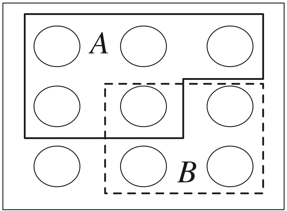
Figure 1.1: A sample space as Pebble World, with two events $A$ and $B$ spotlighted.

1.1.2 De Morgan’s laws

\[ (A\cup B)^c = A^c\cap B^c \]

\[ (A\cap B)^c = A^c\cup B^c \]

since saying that it is not the case that at least one of $A$ and $B$ occur is the same as saying that $A$ does not occur and $B$ does not occur, and saying that it is not the case that both occur is the same as saying that at least one does not occur.

1.1.3 Naive Definition of Probability

Definition 1.3.1 Let $A$ be an event for experiment with a finite sample space $S$. The naive probability of $A$ is

\[ P_{\rm naive}(A)=\frac{|A|}{|S|}=\frac{\mbox{number of outcomes favorable to}\; A}{\mbox{total number of outcomes in}\; S}. \]

This naive definition applies when

there is symmetry in the problem that makes outcomes equally likely (fair coin, standard deck of cards).
the outcomes are equally likely by design. E.g., in simple random sampling, $n$ people are selected randomly with all subsets of size $n$ being equally likely.

How to count?

Now look at Figure 1.1.

To compute $P_{\rm naive}(A)$, we need to count two things:

the number of pebbles in $A$
the number of pebbles in $S$.

These numbers may be very large.

1.1.4 Multiplication rule

Consider a compound experiment consisting of 2 sub-experiments, Experiment A and experiment B.

Suppose that Experiment A has $a$ possible outcomes, and for each of those outcomes, Experiment B has $b$ outcomes.

Then the compound experiment has $ab$ possible outcomes.

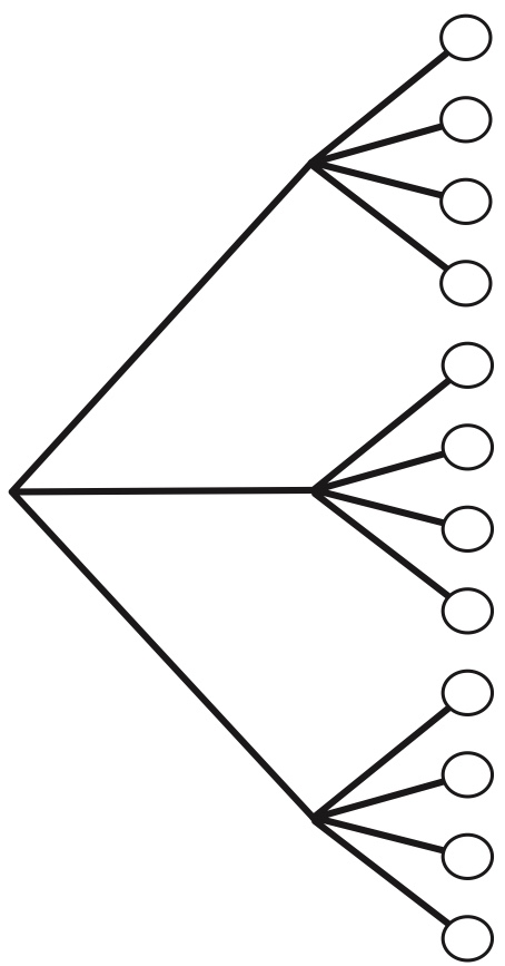
Tree diagram illustrating the multiplication rule. If Experiment $A$ has $3$ possible outcomes, for each of which Experiment $B$ has $4$ possible outcomes, then overall there are $3 imes 4 = 12$ possible outcomes.

Figure 1.2: Tree diagram illustrating the multiplication rule. If Experiment $A$ has $3$ possible outcomes, for each of which Experiment $B$ has $4$ possible outcomes, then overall there are $3 imes 4 = 12$ possible outcomes.

1.1.5 Permutation

The permutation formula is used to calculate the number of ordered arrangements from a set of objects.

If you have $n$ distinct objects and want to arrange $r$ of them (order matters):

\[ P(n, r) = \frac{n!}{(n-r)!} \]

$n!$ (n factorial) = $n \times (n-1) \times (n-2) \times \dots \times 1$
$(n-r)!$ accounts for the unused objects.

If $r = n$:

\[ P(n, n) = n! \]

1.1.6 Combination

The combination formula is used to calculate the number of ways to choose objects from a set when order does not matter.

If you have n distinct objects and want to choose r of them (order does not matter):

\[ C(n, r) = \binom{n}{r} = \frac{n!}{r!(n-r)!} \]

$n!$ (n factorial) = $n \times (n-1) \times (n-2) \times \dots \times 1$
$r!$ accounts for rearrangements of the chosen items.
$(n-r)!$ accounts for the unused objects.

If $r = n$:

\[ C(n, n) = 1 \]

If $r = 0$:

\[ C(n, 0) = 1 \]

1.1.7 Adjustment of overcounting

We can see that \[ C(n, r)=\frac{P(n, r)}{r!} \] The $r!$ accounts for the adjustment of overcounting.

When we calculate: \[ P(n, r) = \frac{n!}{(n-r)!} \] we are counting arrangements of $r$ objects from $n$.

Example: choosing 3 letters (A, B, C) gives us $3! = 6$ different orders:

But combinations ignore order. In combinations, (ABC) is the same as (CAB) or (BCA). They all represent one group of letters, not six different ones.

Every unique combination has been counted $r!$ times in the permutation formula, once for each possible order.

To correct this overcounting, we divide by $r!$:

\[ C(n, r) = \frac{P(n, r)}{r!} = \frac{n!}{r!(n-r)!} \]

1.1.8 Binomial coefficient

For any nonnegative integers $k$ and $n$, the binomial coefficient ${n\choose k}$ is the number of subsets of size $k$ for a set of size $n$.

For $k\leq n$, \[ {n\choose k}=\frac{n(n-1)\cdots (n-k+1)}{k!}=\frac{n!}{(n-k)! k!}. \] For $k>n$, ${n\choose k}=0$.

A binomial coefficient counts the number of subsets of a certain size for a set, such as the number of ways to choose a committee of size $k$ from a set of $n$ people.
Sets and subsets are by definition unordered, e.g., $\{ 3 , 1 , 4 \} = \{ 4 , 1 , 3 \}$, so we are counting the number of ways to choose $k$ objects out of $n$, without replacement and without distinguishing between the different orders in which they could be chosen.

1.1.9 Binomial theorem

The binomial theorem states that

\[ (x+y)^n =\sum_{k=0}^n {n\choose k} x^k y^{n-k}. \]

1.1.10 Sampling with replacement

Consider $n$ objects and making $k$ choices from them, one at a time with replacement. Then there are $n^k$ possible outcomes.

1.1.11 Sampling without replacement

Consider $n$ objects and making $k$ choices from them, one at a time without replacement. Then there are $n(n-1)(n-2)\cdots (n-k+1)$ possible outcomes, for $k\leq n$ (and 0 possibilities for $k>n$).

1.1.12 General definition of probability

A probability space consists of a sample space $S$ and a probability function $P$ which takes an event $A \subseteq S$ as input and returns $P(A)$, a real number between 0 and 1, as output. The function $P$ must satisfy the following ==axioms==:

$P(\emptyset)=0$,
$P(S)=1$，
If $A_1,A_2, \ldots$ are disjoint events, then

\[ P\Bigl(\bigcup_{j=1}^\infty A_j\Bigr)=\sum_{j=1}^\infty P(A_j). \]

(Saying that these events are disjoint means that they are mutually exclusive: $A_i \cap A_j =\emptyset$ for $i\ne j$.)

1.1.13 Properties of probability

Probability has the following properties, for any events $A$ and $B$.

$P(A^c)=1-P(A)$.
If $A \subseteq B$, then $P(A)\leq P(B)$.
$P(A\cup B)=P(A)+P(B)-P(A \cap B)$.

Theorem 1.6.3 (Inclusion-exclusion). For any events $A_1,\ldots,A_n$, \[ \renewcommand{\arraystretch}{1.5} \begin{array}{lll} P\Bigl(\bigcup_{i=1}^n A_i\Bigr) & = & \sum_i P(A_i)-\sum_{i<j}P(A_i \cap A_j) + \\ && \sum_{i<j<k} P(A_i\cap A_j \cap A_k)-\ldots + \\ && (-1)^{n+1} P(A_1\cap\ldots\cap A_n) . \end{array} \renewcommand{\arraystretch}{1} \]

1.2 Examples

1.2.1 Example 1.2.2 (Coin flips).

A coin is flipped 10 times. Writing Heads as $H$ and Tails as $T$, a possible outcome (pebble) is $HHHTHHTTHT$, and the sample space is the set of all possible strings of length 10 of $H$’s and $T$’s. We can (and will) encode $H$ as 1 and $T$ as 0, so that an outcome is a sequence $(s_1,\ldots,s_{10})$ with $s_j \in \{0,1\}$, and the sample space is the set of all such sequences. Now let’s look at some events:

topic: Sample space and event

Let $A_1$ be the event that the first flip is Heads. As a set,

\[ A_1 = \{(1, s_2, \ldots, s_{10}) : s_j \in \{0,1\} \ \text{for } 2 \leq j \leq 10\}. \]

This is a subset of the sample space, so it is indeed an event; saying that $A_1$ occurs is the same thing as saying that the first flip is Heads. Similarly, let $A_j$ be the event that the $j$th flip is Heads for $j = 2, 3, \ldots, 10$.

Let $B$ be the event that at least one flip was Heads. As a set,

\[ B = \bigcup_{j=1}^{10} A_j. \]

Let $C$ be the event that all the flips were Heads. As a set,

\[ C = \bigcap_{j=1}^{10} A_j. \]

Let $D$ be the event that there were at least two consecutive Heads. As a set,

\[ D = \bigcup_{j=1}^{9} \left( A_j \cap A_{j+1} \right). \]

1.2.2 Example 1.2.3 (Pick a card, any card).

Pick a card from a standard deck of 52 cards. The sample space $S$ is the set of all 52 cards (so there are 52 pebbles, one for each card). Consider the following four events:

$A$: card is an ace.
$B$: card has a black suit.
$D$: card is a diamond.
$H$: card is a heart.

topic: Sample space event, and set theory

As a set, $H$ consists of 13 cards:

\[ \{ \text{Ace of Hearts, Two of Hearts, } \ldots, \text{ King of Hearts} \}. \]

We can create various other events in terms of the events $A, B, D,$ and $H$. Unions, intersections, and complements are especially useful for this. For example:

$A \cap H$ is the event that the card is the Ace of Hearts.
$A \cap B$ is the event $\{\text{Ace of Spades, Ace of Clubs}\}$.
$A \cup D \cup H$ is the event that the card is red or an ace.
$(A \cup B)^c = A^c \cap B^c$ is the event that the card is a red non-ace.

Also, note that

\[ (D \cup H)^c = D^c \cap H^c = B, \]

so $B$ can be expressed in terms of $D$ and $H$.

On the other hand, the event that the card is a spade can’t be written in terms of $A, B, D, H$ since none of them are fine-grained enough to distinguish between spades and clubs.

1.2.3 Example 1.4.3 (Runners).

Suppose that 10 people are running a race. Assume that ties are not possible and that all 10 will complete the race, so there will be well-defined first place, second place, and third place winners. How many possibilities are there for the first, second, and third place winners?

topic: Multiplication rule

There are $10$ possibilities for who gets first place, then once that is fixed there are 9 possibilities for who gets second place, and once these are both fixed, there are 8 possibilities for third place. So by the multiplication rule, there are $10 · 9 · 8 = 720$ possibilities.

1.2.4 Example 1.4.5 (Ice cream cones)

Suppose you are buying an ice cream cone. You can choose whether to have a cake cone or a waffle cone, and whether to have chocolate, vanilla, or strawberry as your flavor.

This decision process can be visualized with a tree diagram, as in Figure 1.3.

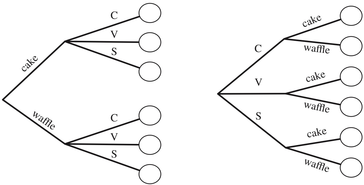
Tree diagram for choosing an ice cream cone. Regardless of whether the type of cone or the flavor is chosen first, there are $2 · 3 = 3 · 2 = 6$ possibilities.

Figure 1.3: Tree diagram for choosing an ice cream cone. Regardless of whether the type of cone or the flavor is chosen first, there are $2 · 3 = 3 · 2 = 6$ possibilities.

How many possible choices do you have to buy a single icecream?

topic: Multiplication rule

We have $2$ options for the cone and $3$ options for the flavor, so we have \[ 2\times 3 =6 \] choices if we buy only one ice cream.

We can label them as

1=Cake+chocolate

2=Cake+vanilla

3=Cake+strawberry

4=Waffle+chocolate

5=Waffle+vanilla

6=Waffle+strawberry

Now suppose you buy two ice cream cones on a certain day, one in the afternoon and the other in the evening. For example, (cakeC, waffleV) to mean a cake cone with chocolate in the afternoon, followed by a waffle cone with vanilla in the evening. How many possible choices do you have?

topic: Multiplication rule and permutation

In the afternoon, we have $6$ options. In the evening, we also have $6$ options. Thus, by multiplication rule, we have \[ 6 \times 6=36 \] ways to buy two icecreams for the afternoon and evening, respectively. The combination can be illustrated with table (the first index is for afternoon and the second index is for evening):

	1	2	3	4	5	6
1	(1,1)	(1,2)	(1,3)	(1,4)	(1,5)	(1,6)
2	(2,1)	(2,2)	(2,3)	(2,4)	(2,5)	(2,6)
3	(3,1)	(3,2)	(3,3)	(3,4)	(3,5)	(3,6)
4	(4,1)	(4,2)	(4,3)	(4,4)	(4,5)	(4,6)
5	(5,1)	(5,2)	(5,3)	(5,4)	(5,5)	(5,6)
6	(6,1)	(6,2)	(6,3)	(6,4)	(6,5)	(6,6)

if you’re only interested in what kinds of ice cream cones you had that day, not the order in which you had them, so you don’t want to distinguish, for example, between (cakeC, waffleV) and (waffleV, cakeC)? Are there now $36/2 = 18$ possibilities?

topic: Multiplication rule, combination and adjusting overcounting

Now $(1, 2)$ and $(2, 1)$ from the table are taken as the same, so are other pairs with the same elements.

However, we need to realize that not all the choices occurred twice in the table. All those diagonal ones, $(1,1), \ldots, (6, 6)$ only occurred once.

So the correct answer is \[ \frac{6\times 5}{2}+6 \]

1.2.5 Example 1.4.6 (Subsets).

How many subsets does a set with $n$ elements have?

\[ 2^n \]

1.2.6 Example 1.4.10 (Birthday problem)

There are $k$ people in a room.
Assume:
- each person’s birthday is equally likely to be any of the 365 days of the year.
- people’s birthdays are independent.
What is the probability that 2 or more people in the group have the same birthday?

Step 1: count possible outcomes in the sample space.

There are $365^k$ ways to assign birthdays to the people in the room, since we can imagine the 365 days of the year being sampled $k$ times, with replacement. By assumption, all of these possibilities are equally likely, so the naive definition of probability applies.

Step 2: count possible outcomes in the event

we just need to count the number of ways to assign birthdays to $k$ people such that there are two people who share a birthday.

Instead, let’s count the complement: the number of ways to assign birthdays to $k$ people such that no two people share a birthday. This amounts to sampling the 365 days of the year without replacement, so the number of possibilities is

\[ 365 \cdot 364 \cdot 363 \cdots (365 - k + 1), \quad \text{for } k \leq 365. \]

Therefore the probability of no birthday matches in a group of $k$ people is

\[ P(\text{no birthday match}) = \frac{365 \cdot 364 \cdot \cdots (365 - k + 1)}{365^k}, \]

and the probability of at least one birthday match is

\[ P(\text{at least 1 birthday match}) = 1 - \frac{365 \cdot 364 \cdot \cdots (365 - k + 1)}{365^k}. \]

1.2.7 Example 1.4.12 (Leibniz’s mistake).

If we roll two fair dice, which is more likely: a sum of $11$ or a sum of $12$?

two outcomes $(5, 6)$ or $(6, 5)$ makes a sum of $11$,

only one outcome $(6, 6)$, makes a sum of $12$

1.2.8 Example 1.4.13 (Committees and teams).

topic: Adjustment of overcounting

Consider a group of four people.

How many ways are there to choose a two-person committee?

Choose 2 from 4, this is a question of combination, so use combination formula: \[ {4\choose 2}=6 \] (b) How many ways are there to break the people into two teams of two people?

The question $b$ looks different with the question $a$, but they are actually from the same process.

If we break people into two distinguishable teams (label these first team as “committee team” and the second team as”regular team”), this is completely equivalent to “select a team of two people as committee”, which is the setting in (a).

In (b), we just do not distinguish two teams with “committee team” and “regular team”.

If we label four people as A B C D, and break them into two team of 2 people, AB|CD and CD|AB are taken as different in question (a), the first one takes AB as committee but the second one uses CD as committee. However, in question (b), AB|CD and CD|AB are the same result, because both of them group AB together and CD together. In other words, each way of partition is counted twice in (a) but only need to be counted once in (b).

From (a), we know there are $6$ ways to select two distinguishable teams, so we just need to adjust the overcounting by dividing $2$, for the answer of (b).

1.2.9 Example 1.4.17 (Club officers)

In a club with n people, there are $n(n - 1)(n - 2)$ ways to choose a president, vice president, and treasurer, and there are
\[ {n\choose 3 }=\frac{n(n - 1)(n - 2)}{3!} \]

ways to choose 3 officers without predetermined titles.

topic: Adjustment of overcounting

1.2.10 Example 1.4.18 (Permutations of a word)

topic: Adjustment of overcounting

Let’s start with a simpler example, how many ways to permutate $AAB$?

First we assume these two $A$s are distinctive, so we denote them as $A_1$ and $A_2$. How many ways to permutate $A_1A_2B$?

We have $3$ unique letters, so we have $3!=6$ permutations, which can be written as \[ A_1A_2B \\ A_2A_1B \\ A_1BA_2 \\ A_2BA_1 \\ BA_1A_2 \\ BA_1A_2 \] However, $A_1$ and $A_2$ are not distinctive in the problem setting, so $A_1A_2B$ and $A_2A_1B$ are over counting’s of the same sequence $AAB$. Since we have $2$ $A$s in the sequence $AAB$, so it got over counted for $2!$ times. The sequence $ABA$ and $BAA$ are also counted for twice. Thus, we only have \[ \frac{3!}{2!}=3 \] ways to permutate $AAB$.

To solve this type of questions,

Step 1: count the total number of letters in the word, and denote it as $n$;

If we assume each letter is unique, we have $n!$ permutations.
Step 2: count the frequency of each letters. In the mini example, $A$ occurs for $n_A=2$ times and $B$ occurs for $n_B=1$ times
Step 3: adjust overcounting by dividing $n!$ by the product of frequencies of each letter \[ \frac{n!}{n_An_B \cdots} \]

How many ways are there to permute the letters in the word LALALAAA?

We have $n=8$ letters in the sequence. Frequencies of letters are $n_L=3$, and $n_A=5$.

Thus, this word can be permutated in \[ \frac{8!}{3!5!} \] ways.

How many ways are there to permute the letters in the word STATISTICS?

Use the same formula, we have

\[ \frac{10!}{3!3!2!} \]

1.2.11 Example 1.4.20 (Full house in poker)

A 5-card hand is dealt from a standard, well-shuffled 52-card deck. The hand is called a full house if it consists of three cards of some rank and two cards of another rank, e.g., three 7’s and two 10’s (in any order). What is the probability of a full house?

topic: Multiplication rule and combination

Step 1: count the total possible outcomes of the sample space, to choose $5$ elements from $52$, we can use the formula of combination, then we have \[ {52\choose 5} \] ways.

To obtain full house, we need $3$ cards from a rank and $2$ cards from another rank. We can break the sampling process into four sub steps:

select the first rank;

(we have $13$ ranks to choose from)
select $3$ cards from the rank we chose;

(Since each rank has $4$ cards, we have ${4\choose 3}$ ways to choose)
select the second rank;

(now we have $12$ ranks to choose from)
select $2$ cards from the second rank we chose;

(we have ${4\choose 2}$ ways)

By the multiplication rule, we have $13{4\choose 3}\times 12{4\choose 2}$ ways to obtain full house.

Now use the naive definition of probability, \[ P(\text{full house})=\frac{13{4\choose 3}\times 12{4\choose 2}}{{52\choose 5}} \]

1.2.12 Example 1.4.21 (Newton-Pepys problem)

topic: set theory and the naive definition of probability

Isaac Newton was consulted about the following problem by Samuel Pepys, who wanted the information for gambling purposes. Which of the following events has the highest probability?

A: At least one 6 appears when 6 fair dice are rolled. \[ P(A)=1-P(\text{no 6 appears})=1-\frac{5^6}{6^6} \approx 0.6651 \] B: At least two 6’s appear when 12 fair dice are rolled. \[ P(B)=1-P(\text{no 6 or only one 6})=1-\frac{5^{12}+{12\choose 1}* 5^{11}}{6^{12}}\approx 0.6187 \] C: At least three 6’s appear when 18 fair dice are rolled. \[ P(C)=1-P(\text{no 6 or only one 6 or two 6})=1-\frac{5^{18}+18*5^{17}+{18\choose 2}*5^{16}}{6^{18}} \approx 0.5973 \]

1.2.13 Example 1.4.22 (Bose-Einstein)

The classic form of the Bose–Einstein Question is “How many ways are there to distribute $k$ indistinguishable bosons into $n$ energy states?”

If you see distribute indistinguishable objects into distinguishable objects, this is very likely to be a Bose-Einstein question. Such as “How many ways to distribute $k$ identical candies among $n$ children (where some children may get zero)”.

In the textbook, this question is formed by:

How many ways are there to choose $k$ times from a set of $n$ objects with replacement, if order doesn’t matter (we only care about how many times each object was chosen, not the order in which they were chosen)?

In this setting, objects are distinguishable. This can be interpreted as “distribute $k$ hand touches to $n$ objects (some objects are never touched)”.

To solve this problem, we use an simpler isomorphic problem (the same problem in a different guise).

Let us find the number of ways to put $k$ indistinguishable particles into $n$ distinguishable boxes. That is, swapping the particles in any way is not considered a separate outcome.

Any configuration can be encoded as a sequence of |’s and ●’s in a natural way, as illustrated in Figure 1.4.

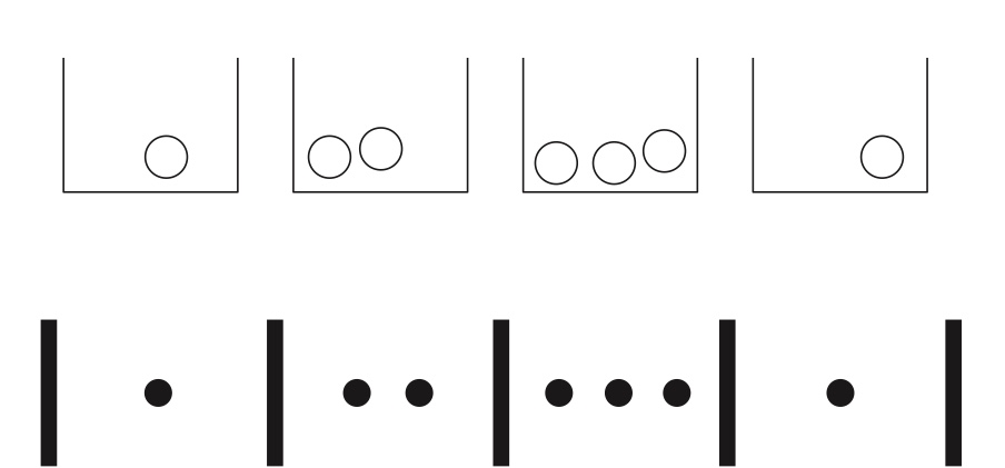
Bose-Einstein encoding: putting $k = 7$ indistinguishable particles into $n = 4$ distinguishable boxes can be expressed as a sequence of $j$’s and $l$’s, where $j$ denotes a wall and $l$ denotes a particle.

Figure 1.4: Bose-Einstein encoding: putting $k = 7$ indistinguishable particles into $n = 4$ distinguishable boxes can be expressed as a sequence of $j$’s and $l$’s, where $j$ denotes a wall and $l$ denotes a particle.

FIGURE 1.6 Bose–Einstein encoding: putting $k=7$ indistinguishable particles into $n=4$ distinguishable boxes can be expressed as a sequence of |’s and ●’s, where | denotes a wall and ● denotes a particle.

To be valid, a sequence must start and end with a |, and have exactly $n-1$ |’s and exactly $k$ ●’s in between the starting and ending |’s; conversely, any such sequence is a valid encoding for some configuration of particles in boxes.

Imagine that we have written down the starting and ending |’s, which represent the outer walls, and in between there are $n+k-1$ fill-in-the-blank slots in between the outer walls.

We need only choose where to put the $k$ ●’s (since then where the $n+k-1$ interior |’s go is completely determined).

So the number of possibilities is

\[ \binom{n+k-1}{k}. \]

This counting method is sometimes called the stars and bars argument, where here we have dots in place of stars.

1.2.14 Example 1.5.1 (Choosing the complement).

For any nonnegative integers $n$ and $k$ with $k\leq n$, we have

\[ {n\choose k}={n\choose n-k}. \]

Story proof: Consider choosing a committee of size $k$ in a group of $n$ people. We know that there are ${n\choose k}$ possibilities. But another way to choose the committee is to specify which $n-k$ people are not on the committee; specifying who is on the committee determines who is not on the committee, and vice versa. So the two sides are equal, as they are two ways of counting the same thing.

1.2.15 Example 1.5.2 (The team captain).

For any positive integers $n$ and $k$ with $k\leq n$, \[ n{n-1 \choose k-1} = k {n\choose k}. \]

Story proof: Consider a group of $n$ people, from which a team of $k$ will be chosen, one of whom will be the team captain. To specify a possibility, we could first choose the team captain and then choose the remaining $k-1$ team members; this gives the left-hand side. Equivalently, we could first choose the $k$ team members and then choose one of them to be captain; this gives the right-hand side.

1.2.16 Example 1.5.3 (Vandermonde’s identity).

A famous relationship between binomial coefficients, called Vandermonde’s identity, says that \[ {m+n \choose k}=\sum_{j=0}^k {m\choose j}{n\choose k-j}. \] Story proof: Consider a group of $m$ men and $n$ women, from which a committee of size $k$ will be chosen. There are ${m+n\choose k}$ possibilities. If there are $j$ men on the committee, then there must be $k-j$ women on the committee. The right-hand side of Vandermonde’s identity sums up the cases for $j$.

1.2.17 Example 1.5.4 (Partnerships).

Let’s use a story proof to show that \[ \frac{(2n)!}{2^n n!}=(2n-1)(2n-3)\cdots 3 \cdot 1. \]

We will show that both sides count the number of ways to break $2n$ people into $n$ partnerships. Take $2n$ people, and give them ID numbers from $1$ to $2n$. We can form partnerships by lining up the people in some order and then saying the first two are a pair, the next two are a pair, etc. This overcounts by a factor of $n! \cdot 2^n$ since the order of pairs doesn’t matter, nor does the order within each pair. Alternatively, count the number of possibilities by noting that there are $2n-1$ choices for the partner of person 1, then $2n-3$ choices for person 2 (or person 3, if person 2 was already paired to person 1), and so on.

1.2.18 Example 1.6.4 (de Montmort’s matching problem).

Consider a well-shuffled deck of $n$ cards, labeled $1$ through $n$. You flip over the cards one by one, saying the numbers $1$ through $n$ as you do so. You win the game if, at some point, the number you say aloud is the same as the number on the card being flipped over (for example, if the 7th card in the deck has the label 7). What is the probability of winning?

Review of Permutations

Imagine there are $n$ people labeled from $1$ to $n$, and $n$ seats also labeled from $1$ to $n$. We randomly assign each person to a seat, meaning the $i$-th person takes the $j$-th seat. Each such assignment corresponds to a permutation, and in total there are $n!$ possible permutations.

In the classic formulation of de Montmort’s matching problem, the seat label represents the number being called, while the card label represents the person.

We can also describe an isomorphic version of the problem: suppose there are $n$ couples, and you are unfamiliar with who belongs to whom. You randomly pair women with men. If at least one true couple is correctly matched, you win. What is the probability of winning?

Solution:

Let $A_i$ be the event that the ith card in the deck has the number i written on it. We are interested in the probability of the union $A_1 \cup \cdots \cup A_n$: as long as at least one of the cards has a number matching its position in the deck, you will win the game.

(An ordering for which you lose is called a derangement, though hopefully no one has ever become deranged due to losing at this game.)

To find the probability of the union, we’ll use inclusion-exclusion. First,

\[ P(A_i) = \frac{1}{n} \] For all $i$. One way to see this is with the naive definition of probability, using the full sample space:
there are $n!$ possible orderings of the deck, all equally likely, and $(n-1)!$ of these are favorable to $A_i$
(fix the card numbered $i$ to be in the $i$th position in the deck, and then the remaining $n-1$ cards can be in any order).

Another way to see this is by symmetry: the card numbered $i$ is equally likely to be in any of the $n$ positions in the deck, so it has probability $1/n$ of being in the $i$th spot.

Second,

\[ P(A_i \cap A_j) \;=\; \frac{(n-2)!}{n!} \;=\; \frac{1}{n(n-1)}, \]

since we require the cards numbered $i$ and $j$ to be in the $i$th and $j$th spots in the deck.

Similarly,

\[ P(A_i \cap A_j \cap A_k) \;=\; \frac{1}{n(n-1)(n-2)}, \]

and the pattern continues for intersections of 4 events, etc. In the inclusion–exclusion formula, there are $n$ terms involving one event, $\binom{n}{2}$ terms involving two events, $\binom{n}{3}$ terms involving three events, and so forth.
By the symmetry of the problem, all $n$ terms of the form $P(A_i)$ are equal, all $\binom{n}{2}$ terms of the form $P(A_i \cap A_j)$ are equal, and the whole expression simplifies considerably:

\[ P\!\left(\bigcup_{i=1}^n A_i \right) = \frac{n}{n} - \frac{\binom{n}{2}}{n(n-1)} + \frac{\binom{n}{3}}{n(n-1)(n-2)} - \cdots + (-1)^{n+1}\cdot \frac{1}{n!}. \]

So,

\[ P\!\left(\bigcup_{i=1}^n A_i \right) = 1 - \frac{1}{2!} + \frac{1}{3!} - \cdots + (-1)^{n+1}\frac{1}{n!}. \]

Comparing this to the Taylor series for $1/e$:

\[ e^{-1} = 1 - \frac{1}{1!} + \frac{1}{2!} - \frac{1}{3!} + \cdots, \]

We see that for large $n$, the probability of winning the game is extremely close to

\[ 1 - \frac{1}{e} \;\approx\; 0.63. \]

Interestingly, as $n$ grows, the probability of winning approaches $1 - \tfrac{1}{e}$ instead of going to $0$ or $1$.

With a lot of cards in the deck, the number of possible locations for matching cards increases, while the probability of any particular match decreases, and these two forces offset each other and balance to give a probability of about $1 - \tfrac{1}{e}$.