3 Essencials of Functions

Understanding Functions is fundamental in mathematics, as they describe the relationship between quantities and form the backbone of calculus, algebra, numerical modeling, and applied sciences. Functions allow us to model change, describe systems, and solve real-world problems [1]–[3].

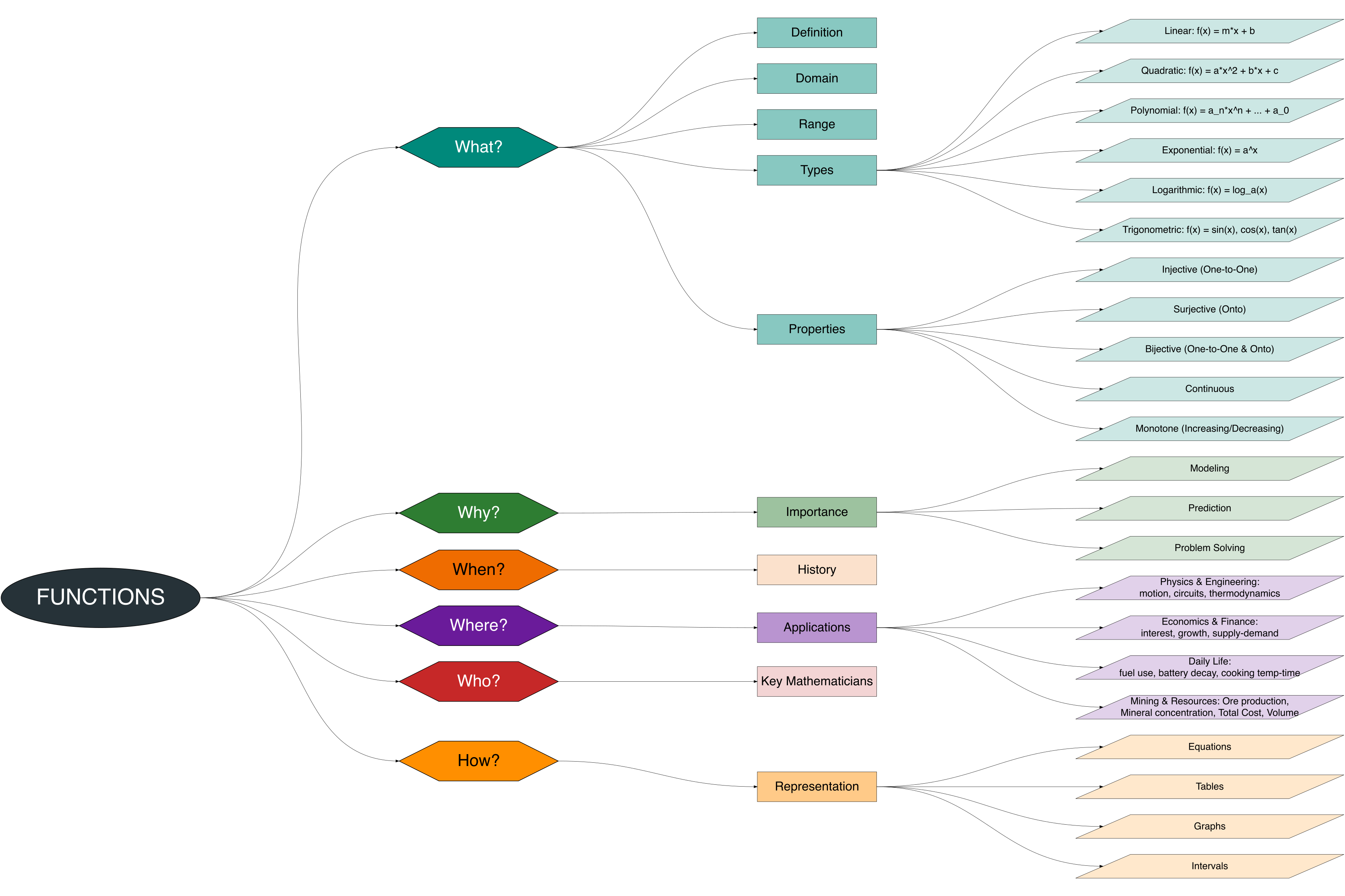
The Figure 3.1 provides a 5W+1H mind map for functions. This visualization guides learners through:

What — definition, domain, range, and types of functions?.
Why — importance and applications in math and science?.
When — historical development and formalization?.
Where — areas of application in engineering, physics, economics, and daily life?.
Who — mathematicians and practitioners using functions?.
How — representation through equations, tables, graphs, and intervals?.

Figure 3.1: Detailed 5W+1H for Functions

Functions are one of the core concepts in mathematics, playing a central role in modeling, analysis, and real-world applications. Using the 5W+1H framework (What, Why, When, Where, Who, How), we can explore functions from multiple perspectives: their definition, importance, historical development, fields of application, key contributors, and different forms of representation.

Table Table 3.1 summarizes the key questions and provides illustrative examples of functions along with their interpretations for each 5W+1H category.

Table 3.1: 5W+1H Questions for Functions

	Description	Example_Function	Example_Output
What?
What?	What is a function?	$f: X \to Y$	Each input → exactly one output
What?	What are the domain and range?	$f(x) = x^2$, Domain = $\mathbb{R}$, Range = $[0,\infty)$	Domain all inputs; Range all outputs
What?	What types of functions exist?	Linear, Quadratic, Polynomial, Exponential, Trigonometric	Example: $f(x)=2x+1$, $f(x)=x^2-3$
What?	What are the key properties of functions?	Injective, Surjective, Bijective, Continuous, Monotone	e.g. $f(x)=x^2$ is not injective on $\mathbb{R}$
Why?
Why?	Why are functions important in mathematics?	Modeling $y=f(x)$ relationships	Predict outcomes, solve equations
Why?	Why do we need to understand function properties?	Analyzing $f(x)$ before applying to problems	Correct manipulation of $f(x)$
When?
When?	When was the function concept formalized?	17th century (Leibniz, Euler)	Formalized in 1600s
When?	When are functions applied in real-life problems?	Finance: $A(t)=P(1+r)^t$; Physics: $s(t)=v_0t+\tfrac12at^2$	Applications in simulations and modeling
Where?
Where?	Where are functions used in science and engineering?	Ohm’s law: $V=IR$, Newton’s law: $F=ma$	Used in circuits, mechanics, chemistry
Where?	Where can functions be observed in economics and daily life?	Population growth $P(t)=P_0e^{rt}$	Used in demand curves, budgeting
Who?
Who?	Who were key mathematicians in developing function theory?	Euler, Leibniz, Dirichlet	Pioneers in function theory
Who?	Who uses functions in practical applications?	Scientists, engineers, economists	Real-world users across disciplines
How?
How?	How are functions represented using equations?	$f(x)=x^2, f(x)=\sin x$	Symbolic form representation
How?	How are functions represented using tables?	Tabular form: $(x,f(x))$ pairs	Input-output lookup
How?	How are functions represented using graphs or intervals?	Graph of $f(x)$, interval $[a,b]$	Visual/geometric representation

3.1 Definition

A function $f$ from set $X$ to set $Y$ is a rule that assigns exactly one element of $Y$ to each element of $X$. Formally:

\[ f: X \to Y \quad \text{such that } \forall x \in X, \exists! y \in Y \text{ with } y = f(x) \]

Domain: the set of all inputs $X$
Range: the set of all outputs $Y$

This definition ensures that every input has one and only one output, which distinguishes functions from more general relations. For example, consider $f(x) = x^2$ with domain $\mathbb{R}$. Each real number $x$ is mapped to a single nonnegative real number $y = x^2$. In this case, the domain is $\mathbb{R}$ and the range is $\mathbb{R}_{\geq 0}$.

3.2 Types of Functions

Functions are fundamental tools in mathematics that describe the relationship between two quantities, typically denoted as an input $x$ and an output $f(x)$. Each type of function has its own characteristics, shape, and application in real-world problems. Understanding these different types of functions is crucial not only in pure mathematics but also in various applied fields such as engineering, economics, physics, and mining engineering, where they are used to model growth, decay, oscillations, and relationships between variables.

Broadly, functions can be categorized into several groups, such as algebraic functions (linear, quadratic, polynomial), transcendental functions (exponential and logarithmic), and trigonometric functions (sine, cosine, tangent).

3.2.1 Algebraic

Algebraic functions (Figure Figure 3.2) are functions that can be expressed using a finite number of algebraic operations such as addition, subtraction, multiplication, division, and raising to a power. These functions form the foundation of many mathematical models and are widely applied in real-life problem solving.

The main types of algebraic functions include:

Linear Function: $f(x) = mx + b$, which produce straight-line graphs and represent constant rates of change.
Quadratic Function: $f(x) = ax^2 + bx + c$, which generate parabolic curves and are often used to model acceleration, projectile motion, or optimization problems.
Polynomial Function: $f(x) = a_n x^n + \dots + a_0$ , which extend the idea of linear and quadratic functions to higher degrees, allowing the modeling of more complex relationships.

Figure 3.2: Algebraic Functions: Linear, Quadratic, and Polynomial (Side by Side)

3.2.2 Transcendental Functions

Transcendental functions (Figure Figure 3.3) are functions that cannot be expressed as finite combinations of algebraic operations. Unlike algebraic functions, they involve processes such as infinite series, exponentiation, and logarithms. These functions play a vital role in describing natural growth, decay, and scaling phenomena.

Exponential Function: $f(x) = a^x$ are used to model rapid growth or decay, such as in population dynamics, radioactive decay, and compound interest.
Logarithmic Function: $f(x) = \log_a x$ serve as the inverse of exponentials, commonly applied in measuring relative change, sound intensity (decibels), pH in chemistry, and data compression in computer science.

Figure 3.3: Exponential and Logarithmic Functions

3.2.3 Trigonometric Functions

The trigonometric functions $f(x) = \sin x, \cos x, \tan x$ describe the relationships between angles and the unit circle. They are fundamental in mathematics, physics, and engineering because they naturally model oscillations, waves, and circular motion. These functions are widely used in areas such as signal processing, alternating current circuits, sound and light waves, and applied fields like surveying and mining for modeling cyclic or repetitive patterns (see Figure Figure 3.4).

Sine ($\sin x$): Range $[-1,1]$, period $2\pi$, zeros at $0^\circ, 180^\circ, 360^\circ$.
Special values: $\sin 30^\circ=\tfrac{1}{2},\ \sin 45^\circ=\tfrac{\sqrt{2}}{2},\ \sin 60^\circ=\tfrac{\sqrt{3}}{2}$
Cosine ($\cos x$): Range $[-1,1]$, period $2\pi$, zeros at $90^\circ, 270^\circ$.
Special values: $\cos 30^\circ=\tfrac{\sqrt{3}}{2},\ \cos 45^\circ=\tfrac{\sqrt{2}}{2},\ \cos 60^\circ=\tfrac{1}{2}$
Tangent ($\tan x$): Period $\pi$, undefined at $90^\circ, 270^\circ$.
Special values: $\tan 30^\circ=\tfrac{1}{\sqrt{3}},\ \tan 45^\circ=1,\ \tan 60^\circ=\sqrt{3}$

Figure 3.4: Trigonometric Functions: sin(x), cos(x), tan(x) with Special Angles

In trigonometry, certain angles are called special angles because their sine, cosine, and tangent values can be expressed in simple radical forms. These angles — such as $0^\circ, 30^\circ, 45^\circ, 60^\circ,$ and $90^\circ$ — are frequently used in mathematics, physics, and engineering for simplifying calculations.

3.3 Properties of Functions

Functions can be understood not only from their formulas, but also from the properties they possess. These properties describe how inputs and outputs are related, and how the function behaves across its domain and codomain (Figure Figure 3.5). Understanding these characteristics helps in identifying whether a function is one-to-one, onto, continuous, or monotone, which are fundamental concepts in both pure and applied mathematics.

Figure 3.5: Function Properties: Injective, Surjective, Bijective, Continuous, Monotone

3.3.1 Injective (One-to-One)

A function is called injective if different inputs always produce different outputs. In other words, no two distinct values in the domain are mapped to the same value in the codomain. For example, $f(x) = 2x + 3$ is injective because every input corresponds to a unique output, whereas $f(x) = x^2$ is not injective over the real numbers, since both $2$ and $-2$ map to the same value, $4$. Understanding injective functions is important in applications where each output must correspond to a unique condition, such as tracking ore quality measurements in mining.

3.3.2 Surjective (Onto)

A function is surjective if every element in the codomain is “covered” by the function, meaning each possible output has at least one pre-image in the domain. For instance, $f(x) = x^3$ from $\mathbb{R}$ to $\mathbb{R}$ is surjective, while $f(x) = e^x$ is not surjective over all real numbers because it cannot produce negative values. Surjective functions are useful when it is essential that all potential outcomes are achievable, such as ensuring full coverage of production or resource allocation scenarios.

3.3.3 Bijective

When a function is both injective and surjective, it is bijective, establishing a perfect one-to-one correspondence between domain and codomain. Every output comes from exactly one input, and an inverse function always exists. For example, $f(x) = x + 5$ is bijective. In practice, bijective functions are valuable in simulations and data transformations, where each output needs to be traced back to a unique input without ambiguity.

3.3.4 Continuous

A function is continuous if its graph can be drawn without lifting the pen. Formally, $f$ is continuous at $x=c$ if $\lim_{x \to c} f(x) = f(c)$. An example is $f(x) = \sin x$, continuous for all real numbers, while $f(x) = 1/x$ is discontinuous at $x=0$. Continuity is crucial for modeling systems with predictable behavior, such as smooth motion of machinery or fluid flow in mining operations.

3.3.5 Monotone

Functions can also be monotone, consistently increasing or decreasing. A monotone increasing function ensures that larger inputs always produce larger outputs, while a monotone decreasing function produces smaller outputs for larger inputs. For example, $f(x) = 2x$ is monotone increasing, while $f(x) = -x$ is monotone decreasing. Monotone functions simplify analysis and optimization, for instance in predicting total ore extracted over time or planning production rates efficiently.

3.4 Applications of Functions

Table 3.2: Applications of Functions in Real Life and Mining

	Description	Example_Function	Example_Output
Science & Engineering
Science & Engineering	Modeling position of moving object	$s(t) = 5t$	At t=3 s → s(3)=15 m
Science & Engineering	Modeling velocity of moving object	$v(t) = 2t$	At t=4 s → v(4)=8 m/s
Economics & Finance
Economics & Finance	Supply-demand curves	$P(x) = 50 + 2x$	Selling 10 items → P(10)=70
Economics & Finance	Compound interest calculation	$A(t) = P(1+r)^t$	Principal $1000, 5% annual, 3 years → $1157.63
Daily Life
Daily Life	Temperature conversion	$F(C) = 9/5 C + 32$	25°C → 77°F
Daily Life	Daily spending tracking	$S(d) = 10d + 5$	Day 7 → $75
Mining & Resources
Mining & Resources	Ore production rate	$Q(t) = 1000 + 50t$	After 5 days → Q(5)=1250 tons
Mining & Resources	Mineral concentration	$C(x) = 0.8x + 5$	x=10 → C(10)=13%
Mining & Resources	Operational cost	$Cost(q) = 5000 + 20q$	Produce 100 units → Cost(100)=$7000
Mining & Resources	Heap volume	$V(A) = 2A + 100$	Area=50 m² → V(50)=200 m³

[1]

Rudin, W., Principles of mathematical analysis, McGraw-Hill, New York, 1976

[2]

Stewart, J., Calculus: Early transcendentals, Cengage Learning, Boston, 2015

[3]

Thomas, G. B., Hass, J. R., Heil, C. E., and Weir, M. D., Thomas’ calculus, Pearson, Boston, 2018