Chapter 7 Wages HW
7.1 Introduction
In this assignment, I worked as a data scientist for the Wage Analytics Division (WAD). I was tasked with determining which demographic and employment characteristics predicted whether a worker earned a high wage or low wage.
7.3 Create the Wage Category Variable
data("Wage")
median_wage <- median(Wage$wage, na.rm = TRUE)
Wage$WageCategory <- ifelse(Wage$wage > median_wage,
                            "High",
                            "Low")
Wage$WageCategory <- factor(Wage$WageCategory,
                            levels = c("Low", "High"))
table(Wage$WageCategory)
##
## Low High
## 1517 14837.5 Classical Statistics Tests
##
##  Welch Two Sample t-test
##
## data:  age by WageCategory
## t = -10.888, df = 2855, p-value < 2.2e-16
## alternative hypothesis: true difference in means between group Low and group High is not equal to 0
## 95 percent confidence interval:
##  -5.298535 -3.681416
## sample estimates:
##  mean in group Low mean in group High
##           40.19512           44.68510
An independent-samples t-test compared the mean age of high wage earners (44.69 years) and low wage earners (40.20). The difference was statistically significant, t(2855) = -10.888, p < .001.
##               Df  Sum Sq Mean Sq F value Pr(>F)
## jobclass       1  223538  223538   134.1 <2e-16 ***
## Residuals   2998 4998547    1667
## ---
## Signif. codes:  0 '***' 0.001 '**' 0.01 '*' 0.05 '.' 0.1 ' ' 1
A one-way ANOVA was conducted to examine whether mean wage differs by job class. The analysis showed a significant effect of job class on wage, F(1, 2998) = 134.1, p < .001.
##
##                  Low High
##   Divorced       118   86
##   Married        872 1202
##   Never Married  479  169
##   Separated       37   18
## Widowed 11 8##
## Pearson's Chi-squared test
##
## data: contingtabmarit
## X-squared = 212.51, df = 4, p-value < 2.2e-16A Chi-square test of independence was conducted to examine whether marital status is associated with wage category. The test showed a significant relationship between the two variables, χ²(4) = 212.51, p < .001. In general, far more high wage earners seem to be married. This association may be due to the fact that the psychological/financial benefits of marriage allow individuals to invest more energy into their work. But, this theory is merely speculative.
n <- sum(contingtabmarit)
chi_sq <- as.numeric(chitest$statistic)
r <- nrow(contingtabmarit)
c <- ncol(contingtabmarit)

cramers_v <- sqrt(chi_sq / (n * (min(r - 1, c - 1))))
cramers_v
## [1] 0.2661507Cramer’s V is .27, meaning that the effect size of the association between marital status and wage is small.
7.6 Logistic Regression Model
set.seed(42)
split <- sample.split(Wage$WageCategory, SplitRatio = 0.7)

training <- subset(Wage, split == TRUE)
testing  <- subset(Wage, split == FALSE)

log_model <- glm(
  WageCategory ~ age + maritl + education + health,
  data = training,
  family = binomial
)

summary(log_model)
##
## Call:
## glm(formula = WageCategory ~ age + maritl + education + health,
## family = binomial, data = training)
##
## Coefficients:
## Estimate Std. Error z value Pr(>|z|)
## (Intercept) -3.255861 0.373442 -8.719 < 2e-16 ***
## age 0.022625 0.004982 4.541 5.59e-06 ***
## maritlMarried 0.820208 0.194407 4.219 2.45e-05 ***
## maritlNever Married -0.416023 0.228951 -1.817 0.06920 .
## maritlSeparated 0.366011 0.426568 0.858 0.39087
## maritlWidowed 0.613146 0.622860 0.984 0.32492
## educationAdvanced Degree 3.052436 0.250998 12.161 < 2e-16 ***
## educationCollege Grad 2.200286 0.219710 10.015 < 2e-16 ***
## educationHS Grad 0.726159 0.211044 3.441 0.00058 ***
## educationSome College 1.518352 0.217545 6.979 2.96e-12 ***
## health>=Very Good 0.367377 0.113967 3.224 0.00127 **
## ---
## Signif. codes: 0 '***' 0.001 '**' 0.01 '*' 0.05 '.' 0.1 ' ' 1
##
## (Dispersion parameter for binomial family taken to be 1)
##
## Null deviance: 2910.9 on 2099 degrees of freedom
## Residual deviance: 2352.7 on 2089 degrees of freedom
## AIC: 2374.7
##
## Number of Fisher Scoring iterations: 4## (Intercept) age maritlMarried
## 0.03854761 1.02288254 2.27097152
## maritlNever Married maritlSeparated maritlWidowed
## 0.65966539 1.44197133 1.84622959
## educationAdvanced Degree educationCollege Grad educationHS Grad
## 21.16684800 9.02759400 2.06712472
## educationSome College health>=Very Good
## 4.56469549 1.44394229The logistic regression revealed a variety of significant predictors of wage. Age, “married” marriage status, and all levels of education were significant. Very good health was also a significant predictor. The predictor with the largest effect size was “advanced degree” (OR = 21.7). This was followed by “college grad” (OR = 9.03) and “some college” (OR = 4.6). The OR did not exceed 3 for any of the other predictors. As a result, we can conclude that higher education, in general, is the most meaningful predictor of wages. The most surprising aspect of this result is the fact that “some college” is such a strong predictor. It is unclear whether this category refers to individuals who completed some college then dropped out, or individuals who completed associate’s degrees or followed related, less standard college pathways.
7.7 Model Evaluation on Test Data
pred_probs <- predict(log_model, newdata = testing, type = "response")
pred_class <- ifelse(pred_probs > 0.5, "High", "Low")
pred_class <- factor(pred_class, levels = c("Low", "High"))
conf_mat <- confusionMatrix(pred_class, testing$WageCategory, positive = "High")
conf_mat
## Confusion Matrix and Statistics
##
## Reference
## Prediction Low High
## Low 345 156
## High 110 289
##
## Accuracy : 0.7044
## 95% CI : (0.6734, 0.7341)
## No Information Rate : 0.5056
## P-Value [Acc > NIR] : < 2.2e-16
##
## Kappa : 0.4081
##
## Mcnemar's Test P-Value : 0.005796
##
## Sensitivity : 0.6494
## Specificity : 0.7582
## Pos Pred Value : 0.7243
## Neg Pred Value : 0.6886
## Prevalence : 0.4944
## Detection Rate : 0.3211
## Detection Prevalence : 0.4433
## Balanced Accuracy : 0.7038
##
## 'Positive' Class : High
## roc_obj <- roc(testing$WageCategory, pred_probs)
plot(roc_obj, col = "blue", lwd = 2, main = "ROC Curve")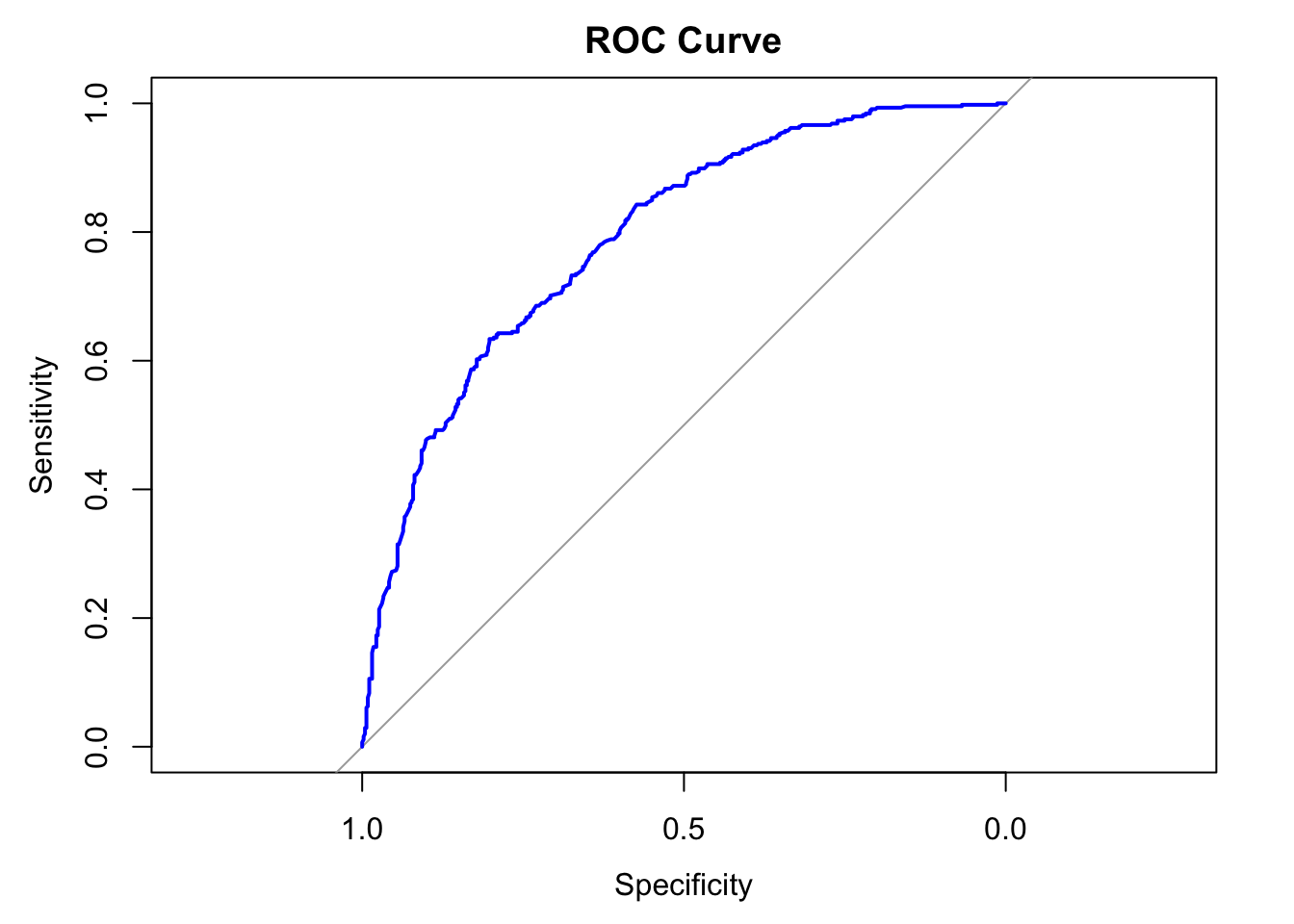
Figure 7.1: ROC Curve
## Area under the curve: 0.7909The accuracy of the model was .70, meaning the model was accurate 70% of the time. This is far better than the No Information Rate of roughly 51% (.5056). The sensitivity of the model was .65, meaning that the model accurately identified true high wage earners as high wage earners 65% of the time. The specificity of model was .76, meaning the model accurately identified true low wage earners as low wage earners 76% of the time. The balanced accuracy (the average of the sensitivity and specificity) was .70. The AUC for the ROC is .7909, meaning that the model has good discrimination ability and will accurately discriminate high wage earners from low wage earners around 79% of the time.
7.8 Final Summary
While education, age, and marital status all relate to wage class, education is clearly the most notable predictor. In particular, advanced degrees are very strong predictors - though the two other classes of college-level education are also far stronger than any other predictors. It is unclear how meaningful the relationship of age, overall marital status, and health are to wage status. These three variables are significant, yet their effect sizes are quite small; further research is needed to determine what their relationships to wage status might be.
Overall, my model performed fairly well on unseen data. The accuracy of my model was around 70%, whereas the accuracy of the No Information rate was around 51%. The model, though, identified low wage earners far more accurately than it identified high wage earners. If I were to redo this model, I would remove all the non-significant predictors, since this makes the most sense statistically. If I were looking into a specific question, though (such as the role of education), I might experiment with removing all non-education related variables.