Chapter 6 Raster Geospatial Data - Continuous
Raster data are fundamentally different from vector data in that they are referenced to a regular grid of rectangular (usually square) cells. The spatial characteristics of a raster dataset are defined by its spatial resolution (the height and width of each cell) and its origin (typically the upper left corner of the raster grid, which is associated with a location in a coordinate reference system). The raster data format has several advantages and limitations compared to vector data. Continuous variables such as elevation, temperature, and precipitation as well as categorical data such as discrete vegetation types and land cover classes can often be stored and manipulated more efficiently as rasters. However, the raster format can be imprecise and inefficient for point, line, and small polygon features such as plot locations, roads, streams, and water bodies.
The terra package provides a variety of specialized classes and functions for importing, processing, analyzing, and visualizing raster datasets (Hijmans 2022). It is intended to replace the raster package, which has been the main raster data package in R for many years. The data objects and the function syntax in the two packages are very similar, and longtime raster users should find it straightforward to work with terra. However, the terra package contains several major improvements, including faster processing speed for large rasters. To avoid unnecessary confusion, the code in this book is based entirely on the newer terra package. There are several other packages that can handle raster data. For example, the older sp package supports the SpatialGridDataFrame class for gridded datasets and spatstat supports the im class for pixel image objects. However, terra is by far the most flexible and powerful package currently available in R for handling raster data.
library(sf)
library(terra)
library(ggplot2)
6.1 Importing Raster Data
A raster object can be created by calling the rast() function and specifying an external image file as an argument. In this example, a dataset of land surface temperature (LST) measured by the MODIS sensor on board the Terra satellite is imported into R as a raster object. MODIS data, along with many other types of satellite remote sensing products, can be obtained from the United State Geological Survey’s Land Processes Distributed Active Archive Center (https://lpdaac.usgs.gov/).
The resulting object belongs to the SpatRaster class. Invoking the print() function for a raster object provides information about the dimensions of the grid, cell size, geographic location, and other details.
lst <- rast("MOD11A2_2017-07-12.LST_Day_1km.tif")
class(lst)
## [1] "SpatRaster"
## attr(,"package")
## [1] "terra"
lst
## class       : SpatRaster
## dimensions  : 1110, 3902, 1  (nrow, ncol, nlyr)
## resolution  : 0.009009009, 0.009009009  (x, y)
## extent      : -104.4326, -69.27943, 30, 40  (xmin, xmax, ymin, ymax)
## coord. ref. : lon/lat WGS 84 (EPSG:4326)
## source      : MOD11A2_2017-07-12.LST_Day_1km.tif
## name        : MOD11A2_2017-07-12.LST_Day_1km
The summary() function provides information about the statistical distribution of raster values, with the size argument specifying the number of randomly sampled pixels to include in the summary.
summary(lst, size = 1e6)
##  MOD11A2_2017.07.12.LST_Day_1km
##  Min.   :    0
##  1st Qu.:    0
##  Median :14981
##  Mean   : 8321
##  3rd Qu.:15148
##  Max.   :16396
There are a number of helper functions, shown below, that can be used to extract specific characteristics of a SpatRaster object. The ncell(), nrow(), ncol(), and nlyr() functions return the numbers of grid cells, grid rows, grid columns, and raster layers in the dataset. The res() function returns the grid cell size.
ncell(lst)
## [1] 4331220
nrow(lst)
## [1] 1110
ncol(lst)
## [1] 3902
nlyr(lst)
## [1] 1
res(lst)
## [1] 0.009009009 0.009009009
The ext() function returns a SpatExtent object that contains the geographic coordinates of the raster extent. SpatExtent objects can be used to specify the extent of new raster objects or to crop rasters to a new extent.
lst_ext <- ext(lst)
class(lst_ext)
## [1] "SpatExtent"
## attr(,"package")
## [1] "terra"
lst_ext[1:4]
##       xmin       xmax       ymin       ymax
## -104.43258  -69.27943   30.00000   40.00000
The crs() function returns a character string containing details about the coordinate reference system (CRS) of the raster dataset. By default, the output is in well-known text (WKT) format. The parse = TRUE argument parses the output into a vector that is easier to read when printed to the R console.
crs(lst, parse = TRUE)
##  [1] "GEOGCRS[\"WGS 84\","
##  [2] "    DATUM[\"World Geodetic System 1984\","
##  [3] "        ELLIPSOID[\"WGS 84\",6378137,298.257223563,"
##  [4] "            LENGTHUNIT[\"metre\",1]]],"
##  [5] "    PRIMEM[\"Greenwich\",0,"
##  [6] "        ANGLEUNIT[\"degree\",0.0174532925199433]],"
##  [7] "    CS[ellipsoidal,2],"
##  [8] "        AXIS[\"geodetic latitude (Lat)\",north,"
##  [9] "            ORDER[1],"
## [10] "            ANGLEUNIT[\"degree\",0.0174532925199433]],"
## [11] "        AXIS[\"geodetic longitude (Lon)\",east,"
## [12] "            ORDER[2],"
## [13] "            ANGLEUNIT[\"degree\",0.0174532925199433]],"
## [14] "    ID[\"EPSG\",4326]]"
The describe = TRUE argument returns an abbreviated summary that includes the CRS name and European Petroleum Specialty Group (EPSG) code for the CRS. More details on working with coordinate reference systems are provided in Chapter 8.
crs(lst, describe = TRUE)
##     name authority code area         extent
## 1 WGS 84      EPSG 4326 <NA> NA, NA, NA, NA
Each layer in a SpatRaster object has a name. By default, this name is the same as the data file that was used to create the raster. Because file names are often long and difficult to interpret, it is useful to specify more readable layer names. Layer names can be extracted and assigned using the names() function.
names(lst)
## [1] "MOD11A2_2017-07-12.LST_Day_1km"
names(lst) <- c("temperature")
names(lst)
## [1] "temperature"
SpatRaster objects can be modified with various functions and used as input to mathematical expressions. In the LST dataset, missing data are coded as zeroes, and the raw digital numbers must be modified by a scaling factor of 0.02 to convert them into degrees Kelvin. The code below uses the ifel() function, which is analogous to the ifelse() function in base R, to replace zero values in the LST dataset with NA values. The first argument to this function is a logical expression, the second is the value to return where the expression is TRUE, and the third is the value to return where the expression is FALSE. The next expression applies the scaling factor to obtain degrees Kelvin and subtracts a constant to further convert the temperatures from Kelvin to Celsius. In both cases, the calculations are automatically carried out for every grid cell in the raster dataset.
lst <- ifel(lst == 0, NA, lst)
lst_c <- lst * 0.02 - 273.15
summary(lst_c, size = 1e6)
##   temperature
##  Min.   : 9.1
##  1st Qu.:28.0
##  Median :29.6
##  Mean   :30.3
##  3rd Qu.:31.5
##  Max.   :54.8
##  NA's   :452091
The global() function can be used to generate statistical summaries of the pixels in a raster dataset. As demonstrated in Chapter 1, the na.rm argument must be TRUE to ignore missing data in the calculations.
global(lst_c, fun = "mean", na.rm=T)
##                 mean
## temperature 30.28687
global(lst_c, fun = "min", na.rm=T)
##              min
## temperature 1.67
global(lst_c, fun = "max", na.rm=T)
##               max
## temperature 54.77
global(lst_c, fun = "sd", na.rm=T)
##                   sd
## temperature 3.652403
Raster objects can be exported using the writeRaster() function. The format of the exported image is specified using the format argument. Common output formats are GTiff (GeoTiff), ascii (ESRI ASCII text ), CDF, (NetCDF), and HFA (ERDAS Imagine). The overwrite=TRUE argument will replace existing files with the same name.
writeRaster(lst_c,
            filename = "MOD11A2_2017-07-12.LST_Day_1km_DegC.tif",
            filetype="GTiff", overwrite=TRUE )
6.2 Maps of Raster Data
The ggplot() function can be used to make maps with raster data, as well as vector data. However, ggplot() only works with inputs in the form of a data frame and therefore cannot be used to directly map a SpatRaster object. Fortunately, raster objects can be converted to data frames with one row per cell, columns for the x and y coordinates, and columns for one or more attribute that are associated with each cell.
In most situations, data frames are very inefficient for storing raster data. Because raster cells are all the same size and arranged on a regular grid, it is not necessary to record the x and y coordinates of every cell. If the coordinates of just one cell (usually called the origin) are known, then the coordinates of any other cell can be determined automatically based on its relative position in the grid. In a data frame, we are effectively storing a vector representation of the raster dataset where each cell is stored as a separate point feature with its own x and y coordinates. Spatial data in a raster object take up less space and can usually be processed more efficiently than the same data stored as points in a data frame. However, converting rasters to data frames will allow us to use ggplot() for all our maps and charts, and is easier at this stage than learning a different graphing system just for rasters.
Converting raster data to a data frame is straightforward, but requires several lines of code. To automate the process, a custom function can be used. The custom function rasterdf() takes a required argument, x, which is the raster object to convert to a data frame. The code in the function extracts the x and y coordinates and data values from the raster and then combines them into a data frame that contains the coordinates and the data. It also has an optional argument, aggregate, that can be used to downsample the raster resolution before converting. In many situations, the raster dataset may contain more cells than the resolution of the image file or screen that will be used to display the map. Using the aggregate argument to downscale the image before converting can greatly reduce the size of the data frame and speed up the mapping process.
The code below uses the function() function to create a custom function.
rasterdf <- function(x, aggregate = 1) {
  resampleFactor <- aggregate
  inputRaster <- x
  inCols <- ncol(inputRaster)
  inRows <- nrow(inputRaster)
  # Compute numbers of columns and rows in the resampled raster
  resampledRaster <- rast(ncol=(inCols / resampleFactor),
                          nrow=(inRows / resampleFactor),
                          crs = crs(inputRaster))
  # Match to the extent of the original raster
  ext(resampledRaster) <- ext(inputRaster)
  # Resample data on the new raster
  y <- resample(inputRaster,resampledRaster,method='near')
  # Extract cell coordinates into a data frame
  coords <- xyFromCell(y, seq_len(ncell(y)))
  # Extract layer names
  dat <- stack(values(y, dataframe = TRUE))
  # Add names - 'value' for data, 'variable' for different
  # layer names in a multilayer raster
  names(dat) <- c('value', 'variable')
  dat <- cbind(coords, dat)
  dat
}
The result is written to a new object called rasterdf, which belongs to the function class.
class(rasterdf)
## [1] "function"
The custom rasterdf() function can be used to convert a SpatRaster object into a data frame. This function can be used in any script, but the code to create the function must always be run before actually calling the function to convert data. The following code converts the LST raster to a data frame after aggregating the cell values by a factor of three.
lst_df <- rasterdf(lst_c, aggregate = 3)
summary(lst_df)
##        x                 y             value
##  Min.   :-104.42   Min.   :30.01   Min.   :11.23
##  1st Qu.: -95.64   1st Qu.:32.50   1st Qu.:28.05
##  Median : -86.86   Median :35.00   Median :29.55
##  Mean   : -86.86   Mean   :35.00   Mean   :30.29
##  3rd Qu.: -78.07   3rd Qu.:37.50   3rd Qu.:31.53
##  Max.   : -69.29   Max.   :39.99   Max.   :54.77
##                                    NA's   :217276
##         variable
##  temperature:481370
##
##
##
##
##
##
The ggplot() function can now be used to map the LST raster. The geom_raster() function is used with the x and y arguments assigned to the corresponding columns in lst_df. The fill argument is the value column from lst_df, which contains the LST values.
Most of the other ggplot() functions have been covered in previous examples. The coord_sf() function is called with the argument expand = FALSE to eliminate extra space and the edges of the map. The legend.position() argument to the theme() function is used to place the legend at the bottom of the map (Figure 6.1).
ggplot(data = lst_df) +
  geom_raster(aes(x = x,
                  y = y,
                  fill = value)) +
  scale_fill_gradient(name = "Degrees C",
                      low = "yellow",
                      high = "red") +
  coord_sf(expand = FALSE) +
  labs(title = "LST-Adjusted Temperature (Terra Day)",
       x = "longitude",
       y = "latitude") +
  theme(legend.position = "bottom")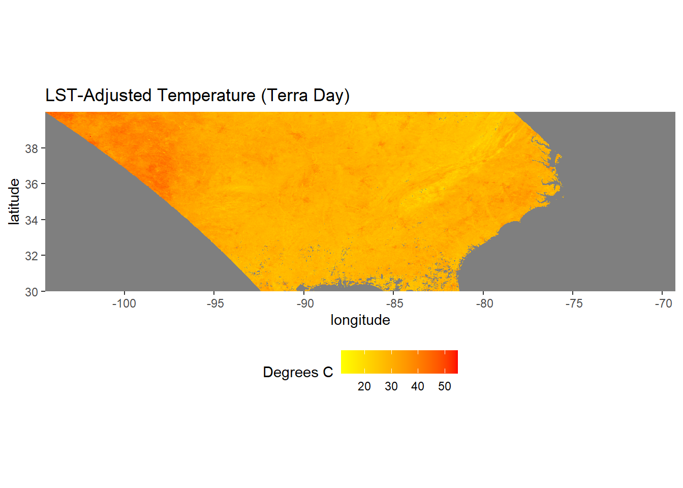
FIGURE 6.1: MODIS Land surface temperature map.
The terra package includes functions for a modifying the geometry of raster datasets. To clip out a smaller portion of the LST dataset, we can use the crop() function. In this example, a bounding box of geographic coordinates (latitude and longitude) is specified to create a SpatExtent object and crop the raster to the U.S. state of Georgia.
clipext <- ext(-86, -80.5, 30, 35.5)
class(clipext)
## [1] "SpatExtent"
## attr(,"package")
## [1] "terra"
lst_clip <- crop(lst_c, clipext)
lst_clip_df <- rasterdf(lst_clip)
There are numerous other terra functions for raster GIS operations, including aggregating and resampling to different cell sizes, focal statistics, and zonal statistics. Many of these functions will be demonstrated in the upcoming chapters
Often, it is helpful to plot boundary features on top of a raster to provide context. Vector and raster data can be combined in ggplot() by using the appropriate geom function for each data type. Here, the Georgia county boundaries are overlaid on the LST raster.
ga_sf <- st_read(dsn = "GA_SHP.shp", quiet = TRUE)To add the county boundaries, the geom_sf() function can be used as in the examples from the previous chapter. The fill = NA argument displays the polygons as a hollow wireframe so that the raster data can be seen underneath (Figure 6.2).
ggplot() +
  geom_raster(data = lst_clip_df,
              aes(x = x,
                  y = y,
                  fill = value)) +
  geom_sf(data=ga_sf,
          color = "grey50",
          fill = NA, size = 0.5) +
  scale_fill_gradient(name = "Degrees C",
                      low = "yellow",
                      high = "red") +
  coord_sf(expand = FALSE) +
  labs(title = "LST-Adjusted Temperature (Terra Day)",
       x = "longitude",
       y = "latitude")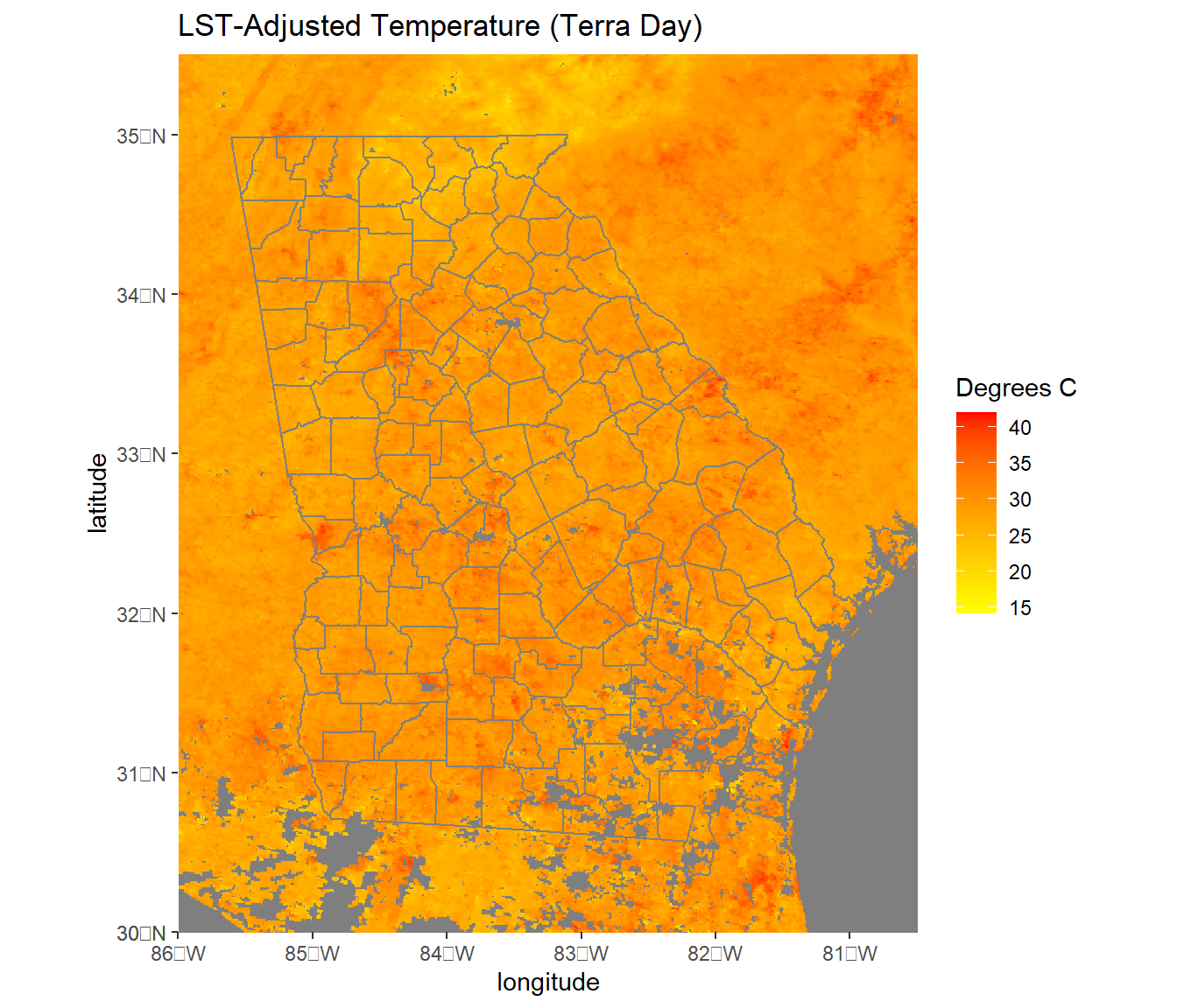
FIGURE 6.2: MODIS Land surface temperature cropped to the state of Georgia with county boundary overlaid.
6.3 Multilayer Rasters
The next examples will use forcings data from the North American Land Data Assimilation System (NLDAS). These are gridded meterological data that can be obtained through the National Aeronautics and Space Administration’s Goddard Earth Sciences Data and Information Services Center (https://disc.gsfc.nasa.gov/). The data have a grid cell size of 0.125 x 0.125 degrees and are stored as GeoTIFF files and can be imported as SpatRaster objects in the same way as the LST dataset.
temp2012 <- rast("NLDAS_FORA0125_M.A201207.002.grb.temp.tif")
temp2013 <- rast("NLDAS_FORA0125_M.A201307.002.grb.temp.tif")
temp2014 <- rast("NLDAS_FORA0125_M.A201407.002.grb.temp.tif")
temp2015 <- rast("NLDAS_FORA0125_M.A201507.002.grb.temp.tif")
temp2016 <- rast("NLDAS_FORA0125_M.A201607.002.grb.temp.tif")
temp2017 <- rast("NLDAS_FORA0125_M.A201707.002.grb.temp.tif")
Multiple SpatRaster objects can be combined to produce multi-layer raster datasets. These objects are frequently used for space-time data because they can store rasters from different dates. Multi-layer rasters are created using the c() (combine) function, similar to the way that this function is used in base R to combine multiple objects into vectors. The following code creates two multi-layer SpatRaster objects, one containing July temperature data from 2012-2017 and one containing July precipitation data from 2012-2017. The names() function is used to specify the layer names for each object.
tempstack <- c(temp2012, temp2013, temp2014,
               temp2015, temp2016, temp2017)
names(tempstack) <- c("July 2012", "July 2013", "July 2014",
                      "July 2015", "July 2016", "July 2017")
Alternatively, multi-layer rasters can be created by making a single call to rast() and providing a vector of file names to import and combine.
tempstack <- rast(c("NLDAS_FORA0125_M.A201207.002.grb.temp.tif",
                    "NLDAS_FORA0125_M.A201307.002.grb.temp.tif",
                    "NLDAS_FORA0125_M.A201407.002.grb.temp.tif",
                    "NLDAS_FORA0125_M.A201507.002.grb.temp.tif",
                    "NLDAS_FORA0125_M.A201607.002.grb.temp.tif",
                    "NLDAS_FORA0125_M.A201707.002.grb.temp.tif"))
names(tempstack) <- c("July 2012", "July 2013", "July 2014",
                      "July 2015", "July 2016", "July 2017")
When the global() function is applied to multi-layer rasters, each layer in the SpatRaster object is summarized individually.
global(tempstack, stat = "mean", na.rm=T)
##               mean
## July 2012 297.8852
## July 2013 296.1879
## July 2014 295.7905
## July 2015 296.2655
## July 2016 296.5719
## July 2017 296.7618
From these summaries, is apparent that the temperature units are in Kelvin. As was done with the MODIS LST data, these data can be converted to Celsius using a simple R expression. The expression is automatically applied to all the layers in the multi-layer SpatRaster object.
tempstack <- tempstack - 273.15
global(tempstack, stat = "mean", na.rm=T)
##               mean
## July 2012 24.73522
## July 2013 23.03793
## July 2014 22.64051
## July 2015 23.11549
## July 2016 23.42190
## July 2017 23.61176
Multi-layer rasters can be mapped using ggplot(). First, the SpatRaster object is converted to a data frame using the custom rasterdf() function, and a dataset of U.S. state boundaries is imported for use as an overlay.
tempstack_df <- rasterdf(tempstack)
summary(tempstack_df)
##        x                 y             value
##  Min.   :-124.94   Min.   :25.06   Min.   : 3.09
##  1st Qu.:-110.47   1st Qu.:32.03   1st Qu.:19.59
##  Median : -96.00   Median :39.00   Median :23.53
##  Mean   : -96.00   Mean   :39.00   Mean   :23.43
##  3rd Qu.: -81.53   3rd Qu.:45.97   3rd Qu.:27.62
##  Max.   : -67.06   Max.   :52.94   Max.   :40.18
##                                    NA's   :140982
##       variable
##  July 2012:103936
##  July 2013:103936
##  July 2014:103936
##  July 2015:103936
##  July 2016:103936
##  July 2017:103936
##
states_sf <- read_sf("conterminous_us_states.shp", quiet = TRUE)
Then, ggplot() is used with facet_wrap() to display a composite plot with one year mapped in each facet. The variable column, which contains the names of the different raster layers, is specified in the facets argument. The temperature data are displayed using a yellow to red color ramp with a vector dataset of state boundaries overlaid to provide a spatial reference (Figure 6.3).
ggplot() +
  geom_raster(data = tempstack_df,
              aes(x = x,
                  y = y,
                  fill = value)) +
  geom_sf(data = states_sf,
          fill = NA,
          color = "grey50",
          size = 0.25) +
  scale_fill_gradient(name = "Degrees C",
                      low = "yellow",
                      high = "red") +
  coord_sf(expand = FALSE) +
  facet_wrap(facets = vars(variable), ncol = 2) +
  labs(title = "Mean July Temperature",
       x = "longitude",
       y = "latitude")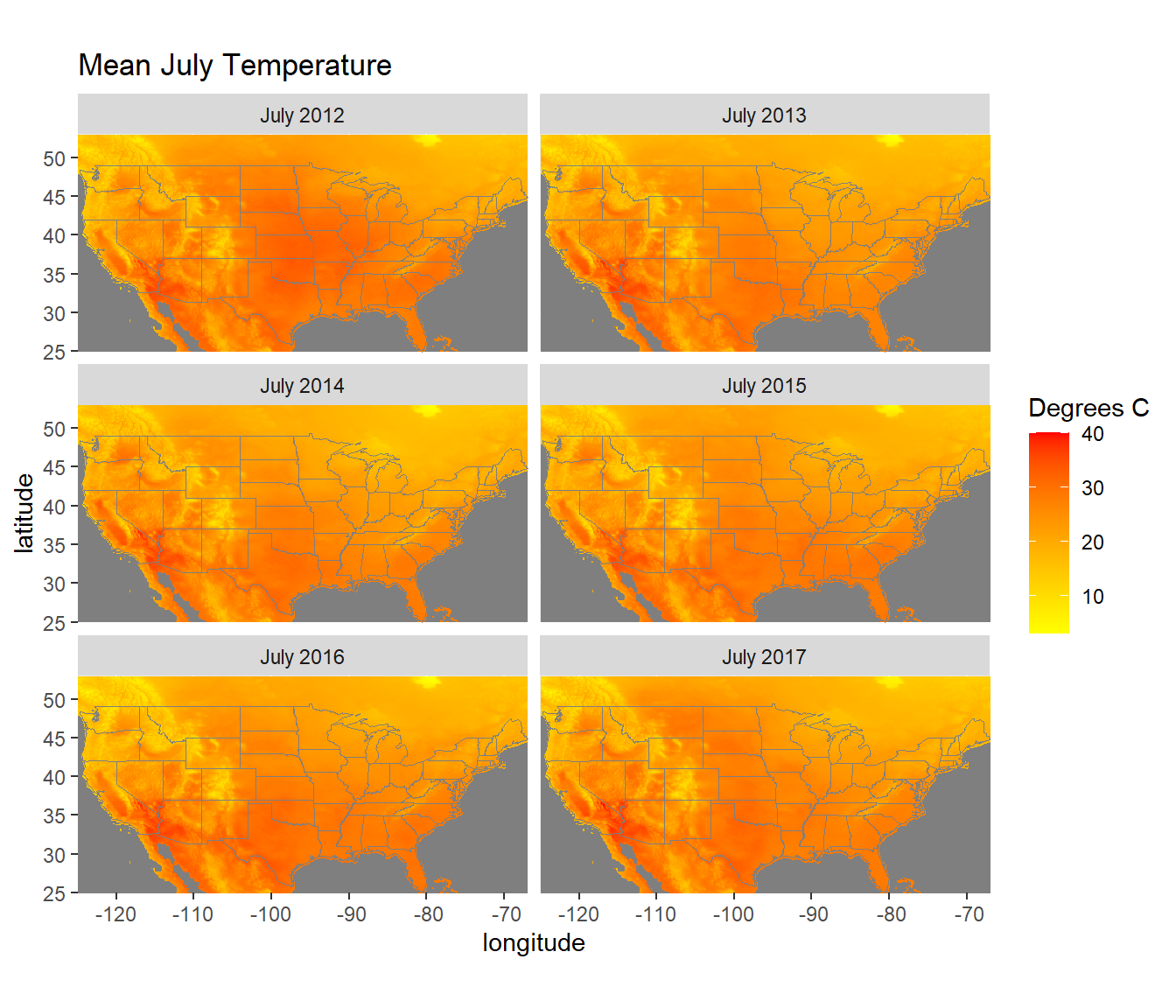
FIGURE 6.3: July temperatures from the NLDAS forcings dataset.
6.4 Computations on Raster Objects
Many statistical summary functions have methods for raster objects. When used with multi-layer rasters, these functions will be applied to each pixel to summarize the data across all layers. For example, the following code generates a mean temperature for each pixel using the six years of data stored in different layers. Note the difference compared to the summaries calculated with global(), which were summarized across all pixels for each layer instead of across all layers for each pixel.
meantemp <- mean(tempstack)As in the previous example, temperature is displayed using a yellow to red color ramp with a vector dataset of state boundaries overlaid (Figure 6.4).
meantemp_df <- rasterdf(meantemp)

ggplot() +
  geom_raster(data = meantemp_df, aes(x = x,
                                      y = y,
                                      fill = value)) +
  geom_sf(data = states_sf,
          fill = NA,
          color = "grey50",
          size = 0.25) +
  scale_fill_gradient(name = "Degrees C",
                      low = "yellow",
                      high = "red") +
  coord_sf(expand = FALSE) +
  labs(title = "Mean July Temperature, 2012-2017",
       x = "longitude", y = "latitude") +
  theme(legend.position = "bottom")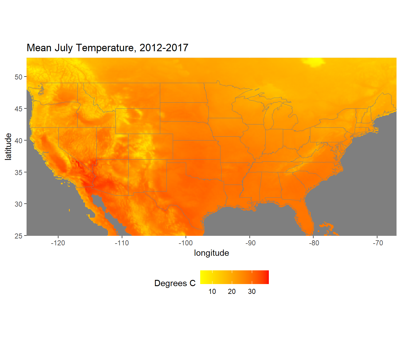
FIGURE 6.4: Mean July temperatures calculated from 2012-2017.
The following code subtracts each of the six annual datasets in the multi-layer raster from the mean temperature layer to generate maps of temperature anomalies. In this example, tempstack is a raster object with six layers, and meantemp is a raster object with one layer. When the subtraction operator is used, meantemp is subtracted from each layer of tempstack, producing a new SpatRaster object with six layers called tempanom. The layer names from tempstack are then assigned to tempanom.
tempanom <- tempstack - meantemp
names(tempanom) <- names(tempstack)
The anomalies are displayed using a bicolor ramp generated with the scale_fill_gradients2() function. This approach is justified because the anomalies have a breakpoint at zero. Positive (warm) anomalies are displayed as red, and negative (cold) anomalies are displayed as blue. By default, the color break is at zero, but this value can be changed by modifying the 'midpoint argument to scale_fill_gradient2(). The theme_void() function is used to remove the axes and graticules from the maps, and the theme() function is used to bold the text labels and increase the font sizes. Using the expand = TRUE argument with coord_df() provides some additional space around the maps and makes their labels easier to read (Figure 6.5).
tempanom_df <- rasterdf(tempanom)

ggplot() +
  geom_raster(data = tempanom_df, aes(x = x,
                                      y = y,
                                      fill = value)) +
  geom_sf(data = states_sf,
          fill = NA,
          color = "grey50",
          size = 0.25) +
  scale_fill_gradient2(name = "Degrees C",
                       low = "blue",
                       mid = "lightyellow",
                       high = "red") +
  coord_sf(expand = TRUE) +
  facet_wrap(facets = vars(variable), ncol = 2) +
  theme_void() +
  theme(strip.text.x = element_text(size=12, face="bold"))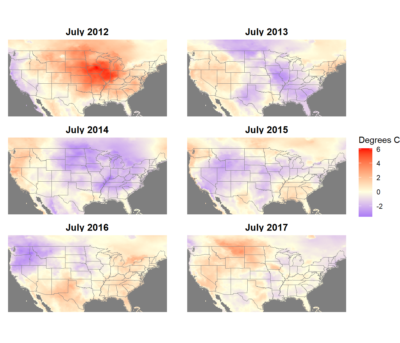
FIGURE 6.5: July temperature anomalies from the NLDAS forcings dataset.
In a most real applications,more than six years of meteorological data (typically 30 years) would be used to generate a mean climatology for calculating anomalies. This small example is presented to illustrate the advantages of converting annual meteorological data into anomalies. The untransformed temperature data show the same strong spatial patterns every year. By subtracting the mean temperature map from each annual temperature map, the spatial pattern of temperature is removed and the interannual variation is emphasized in the anomaly maps.
One or more layers can be extracted from a raster object using double brackets. As with lists in base R, raster layers can be extracted either by number or name.
temp1 <- tempstack[[1]]
names(temp1)
## [1] "July 2012"
temp2 <- tempstack[["July 2012"]]
names(temp2)
## [1] "July 2012"
temp3 <- tempstack[[1:3]]
names(temp3)
## [1] "July 2012" "July 2013" "July 2014"
The terra package has methods for many of the base R plotting functions. This means that a SpatRaster object can be provided as an input to these functions, and R will be able to generate an appropriate map or graph. For example, the generic plot() function is handy for generating a quick map of a raster object (Figure 6.6).
plot(tempstack[[1]])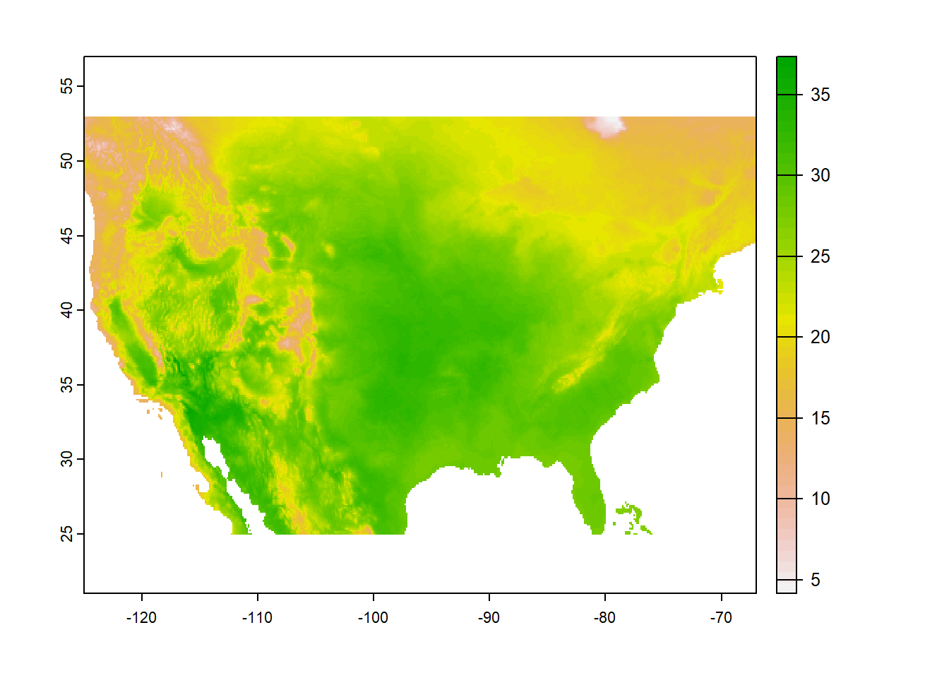
FIGURE 6.6: Raster map created with the generic plot method.
The plot() function will also work with multi-layer rasters, automatically generating a multi-panel figure with one map for each layer (Figure 6.7).
plot(tempstack)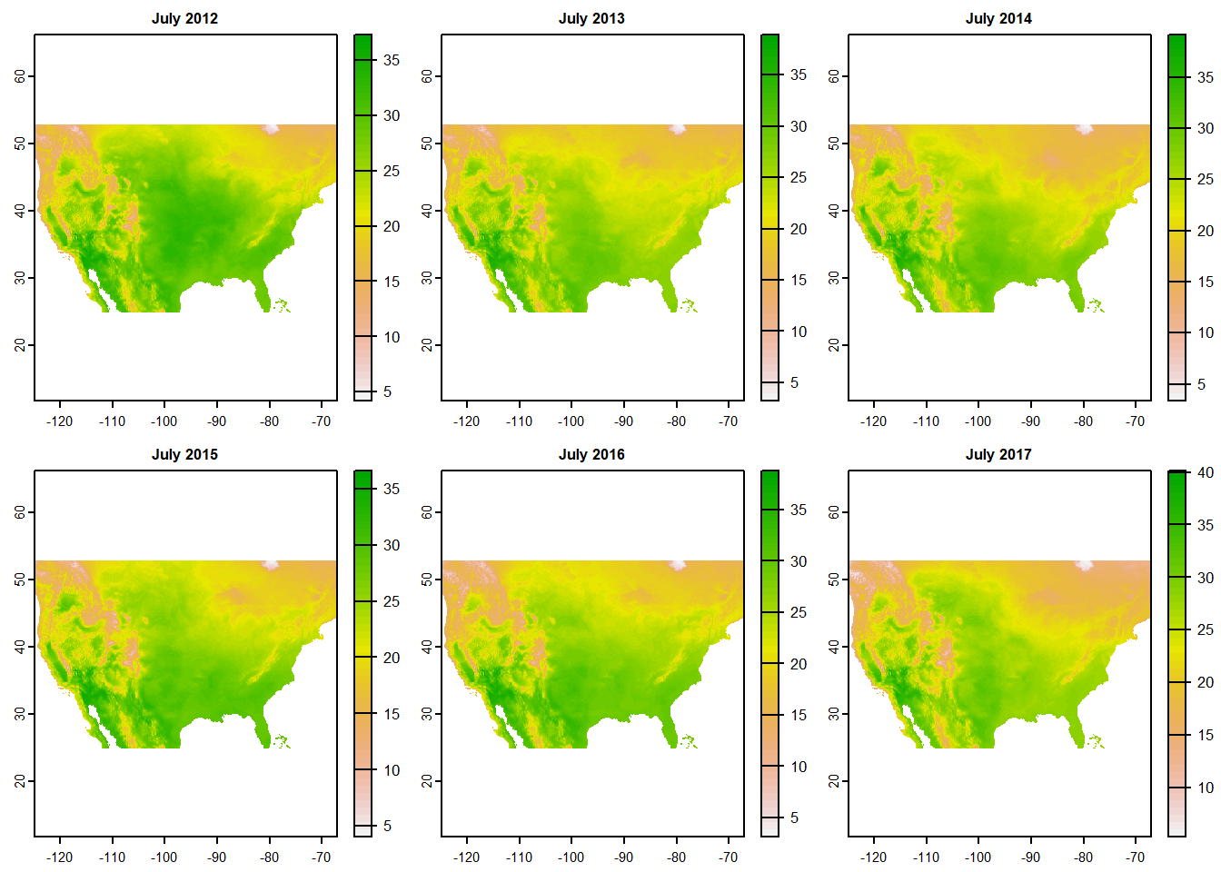
FIGURE 6.7: Multilayer raster map created with the generic plot method.
The hist() function will automatically generate a histogram or density plot for each layer in a raster object (Figure 6.8).
hist(tempstack)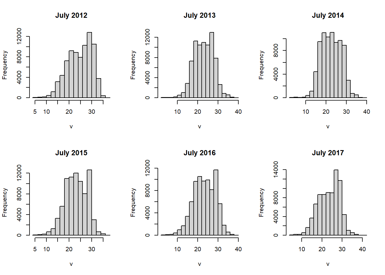
FIGURE 6.8: Histograms of raster layers.
When two single-layer rasters are provided as arguments to the plot() function, it will generate a scatterplot. Because of the large number of cells in most raster datasets, simply plotting them all as points produces a large blob. Setting the gridded=TRUE argument produces a gridded scatterplot, in which the value of each grid cell represents the density of points in that portion of the scatterplot (Figure 6.9).
plot(temp2012, temp2013,
     xlab = "2012",
     ylab = "2013",
     gridded = TRUE)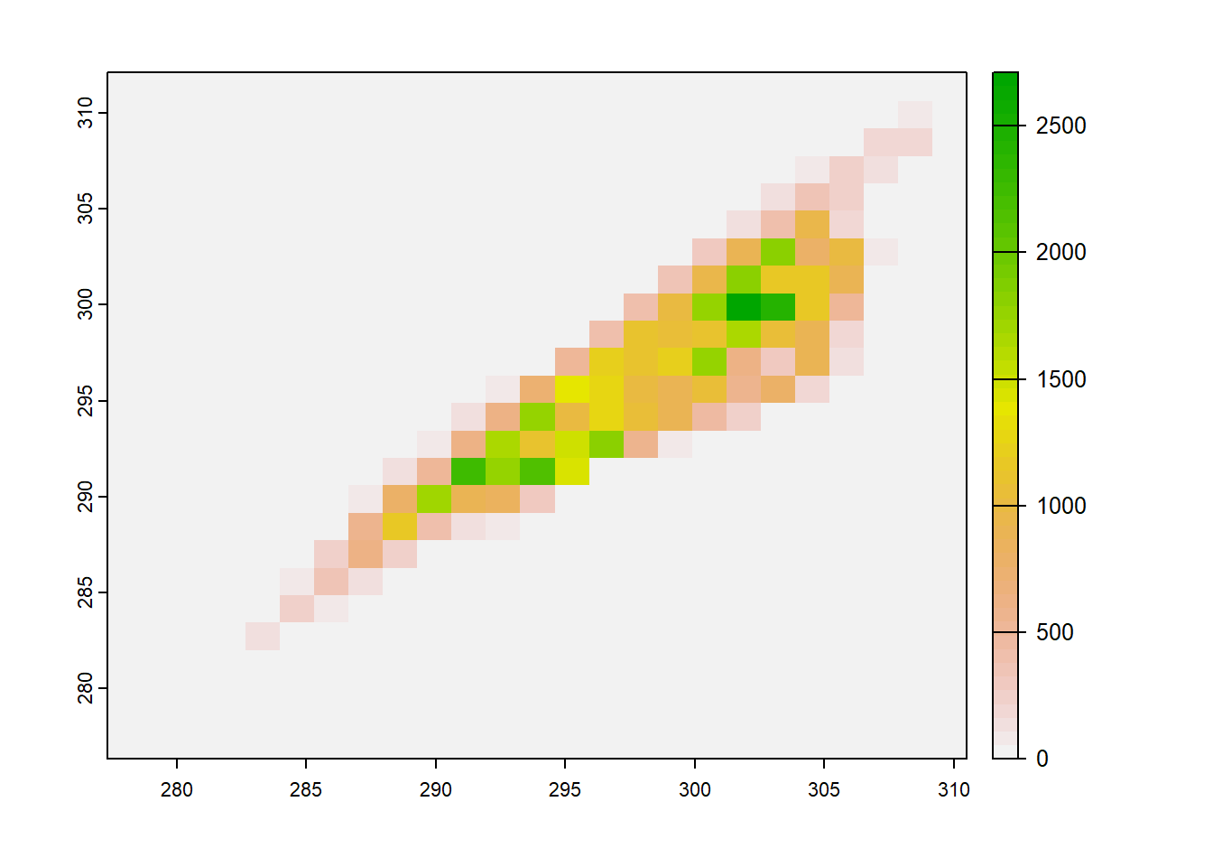
FIGURE 6.9: Gridded scatterplot of two raster datasets.
These functions are very handy for generating quick, interactive visualizations for large raster objects, and it is possible to customize them more if you are familiar with plotting in base R. However, it is also possible to convert raster data into a data frame using rasterdf() and graph it with ggplot() if you want to have more control over the layout of your plot. Several examples of using ggplot() to plot summaries of raster data will be provided in later chapters. There are also a number of specialized mapping packages that work with terra and sf objects, including rasterVis (Perpinan Lamigueiro and Hijmans 2022), tmap (Tennekes 2018), and leaflet (Cheng, Karambelkar, and Xie 2022).
More resources on the terra package can be found at https://rspatial.org/terra/spatial/index.html, including detailed explanations of many functions and examples with a variety of remote sensing datasets. The upcoming second edition of Geocomputation with R by Robin Lovelace and others (Lovelace, Nowosad, and Muenchow 2019) will incorporate the terra packages and should be an excellent reference and source of further examples.
6.5 Practice
Convert the clipped LST raster from Celsius to Fahrenheit and generate an updated version of the Georgia LST map.
Generate a new raster where each pixel contains the standard deviation of the NLDAS July Temperature values from 2012-2017. Map the result to explore where temperatures were most variable over this period.
Create a new raster dataset where each cell contains the difference between July 2015 temperature and July 2016 temperature. Examine the map and histogram of this raster and use them to assess changes in temperature between 2015 and 2016.