Chapter 3 Processing Tabular Data
The preceding chapter provided a foundation for visualizing data using the ggplot2 package. The sample dataset used in the examples was already in a format suitable for plotting with ggplot(). However, in most cases, data need to be reformatted before they can be visualized and analyzed. Common formatting tasks include selecting subsets of rows and columns from the data table, calculating new variables from the raw data values, computing summary statistics, and combining data from different sources.
This tutorial will demonstrate basic functions for manipulating data frames (and tibbles). These manipulations can be accomplished in a variety of ways, including using base R operators and functions like those covered in Chapter 1. However, the functions in the dplyr and tidyr packages provide a more consistent and intuitive approach. These packages (along with the ggplot2, readr, and readxl packages used in Chapter 2) are part of the tidyverse, collection of data science R packages. These packages share an underlying design philosophy, grammar of data manipulation, and set of data structures. The rest of this book will make extensive use of these packages. They will provide the basis for carrying out sophisticated processing, analysis, and visualization of complex “real-world” datasets by writing concise and easily interpretable R code.
To run the examples in this chapter, it is necessary to use the library() function to load the previously-mentioned tidyverse packages. Remember that if these packages are not available on your computer, you will need to install them using the install.packages() function or the installation tools available in RStudio.
library(ggplot2)
library(dplyr)
library(tidyr)
library(readr)
library(readxl)
The tutorials in this chapter will use the same Oklahoma Mesonet dataset that was used in Chapter 2. The output is printed to the console with the glimpse() function. This function shows the first few rows of data from mesosm, with one column from the data frame shown on each row of the printed output. This format makes it easier to see all the variables in the data frame without having the wrap the console output across multiple lines.
mesosm <- read_csv("mesodata_small.csv", show_col_types = FALSE)
glimpse(mesosm)
## Rows: 240
## Columns: 9
## $ MONTH <dbl> 1, 2, 3, 4, 5, 6, 7, 8, 9, 10, 11, 12, 1, 2,…
## $ YEAR  <dbl> 2014, 2014, 2014, 2014, 2014, 2014, 2014, 20…
## $ STID  <chr> "HOOK", "HOOK", "HOOK", "HOOK", "HOOK", "HOO…
## $ TMAX  <dbl> 49.48032, 47.18071, 60.70613, 72.36483, 84.3…
## $ TMIN  <dbl> 17.92903, 17.05357, 26.06806, 39.32103, 48.3…
## $ HMAX  <dbl> 83.04161, 88.28857, 78.96613, 81.82690, 75.3…
## $ HMIN  <dbl> 29.00226, 39.94393, 25.39871, 21.02207, 18.8…
## $ RAIN  <dbl> 0.17, 0.30, 0.31, 0.40, 1.25, 3.18, 2.58, 0.…
## $ DATE  <date> 2014-01-01, 2014-02-01, 2014-03-01, 2014-04…
3.1 Single Table Verbs
Each dplyr function accomplishes a particular type of data transformation. These functions are referred to as “verbs” that describe the action performed. Some dplyr verbs operate on a single data frame or tibble, while others operate by combining data from two or more. Below is a list of some important dplyr verbs for single tables:
select()andrename()select variables (columns) based on their names.filter()selects observations (rows) based on their values.arrange()reorders observations.mutate()andtransmute()add new variables that are functions of existing variables.
The first argument to each function is the data frame that will be modified. Additional comma-separated arguments control how the function will be implemented.
3.1.1 Select and Rename
In the context of dplyr, selecting specifically refers to choosing a subset of the columns within a data frame based on user-specified criteria. The simplest way is to specify the names of the columns to be retained. The select() function returns only the specified columns. Other columns are removed from the data frame. One way to specify the selected columns is a comma-separated list of column names. In the following examples, the outputs are not assigned to a new object, so by default, they are printed to the console.
select(mesosm, STID, YEAR, MONTH, TMAX, TMIN)
## # A tibble: 240 × 5
##    STID   YEAR MONTH  TMAX  TMIN
##    <chr> <dbl> <dbl> <dbl> <dbl>
##  1 HOOK   2014     1  49.5  17.9
##  2 HOOK   2014     2  47.2  17.1
##  3 HOOK   2014     3  60.7  26.1
##  4 HOOK   2014     4  72.4  39.3
##  5 HOOK   2014     5  84.4  48.3
##  6 HOOK   2014     6  90.7  61.9
##  7 HOOK   2014     7  90.6  64.7
##  8 HOOK   2014     8  95.8  64.5
##  9 HOOK   2014     9  84.3  58.0
## 10 HOOK   2014    10  76.1  44.9
## # … with 230 more rows
The : operator can be used to select a continuous series of columns. This usage is analogous to the : operator in base R, where it is used to specify a continuous series of integers.
select(mesosm, MONTH:TMAX)
## # A tibble: 240 × 4
##    MONTH  YEAR STID   TMAX
##    <dbl> <dbl> <chr> <dbl>
##  1     1  2014 HOOK   49.5
##  2     2  2014 HOOK   47.2
##  3     3  2014 HOOK   60.7
##  4     4  2014 HOOK   72.4
##  5     5  2014 HOOK   84.4
##  6     6  2014 HOOK   90.7
##  7     7  2014 HOOK   90.6
##  8     8  2014 HOOK   95.8
##  9     9  2014 HOOK   84.3
## 10    10  2014 HOOK   76.1
## # … with 230 more rows
The helper functions starts_with(), ends_with(), and contains() can be used to find multiple columns by matching part of the column name.
select(mesosm, starts_with("T"))
## # A tibble: 240 × 2
##     TMAX  TMIN
##    <dbl> <dbl>
##  1  49.5  17.9
##  2  47.2  17.1
##  3  60.7  26.1
##  4  72.4  39.3
##  5  84.4  48.3
##  6  90.7  61.9
##  7  90.6  64.7
##  8  95.8  64.5
##  9  84.3  58.0
## 10  76.1  44.9
## # … with 230 more rows
Columns can be removed by prefixing their names with a -. Other columns will be kept.
select(mesosm, -HMIN, -HMAX)
## # A tibble: 240 × 7
##    MONTH  YEAR STID   TMAX  TMIN  RAIN DATE
##    <dbl> <dbl> <chr> <dbl> <dbl> <dbl> <date>
##  1     1  2014 HOOK   49.5  17.9  0.17 2014-01-01
##  2     2  2014 HOOK   47.2  17.1  0.3  2014-02-01
##  3     3  2014 HOOK   60.7  26.1  0.31 2014-03-01
##  4     4  2014 HOOK   72.4  39.3  0.4  2014-04-01
##  5     5  2014 HOOK   84.4  48.3  1.25 2014-05-01
##  6     6  2014 HOOK   90.7  61.9  3.18 2014-06-01
##  7     7  2014 HOOK   90.6  64.7  2.58 2014-07-01
##  8     8  2014 HOOK   95.8  64.5  0.95 2014-08-01
##  9     9  2014 HOOK   84.3  58.0  1.48 2014-09-01
## 10    10  2014 HOOK   76.1  44.9  1.72 2014-10-01
## # … with 230 more rows
The rename() function is used to change column names. Name changes are specified using the = operator, placing the new name first and the old name second. After an external dataset has been imported, it is often desirable to change the names of the columns to make them shorter, more interpretable, or more consistent with other column names.
rename(mesosm, maxtemp = TMAX, mintemp = TMIN)
## # A tibble: 240 × 9
##    MONTH  YEAR STID  maxtemp mintemp  HMAX  HMIN  RAIN
##    <dbl> <dbl> <chr>   <dbl>   <dbl> <dbl> <dbl> <dbl>
##  1     1  2014 HOOK     49.5    17.9  83.0  29.0  0.17
##  2     2  2014 HOOK     47.2    17.1  88.3  39.9  0.3
##  3     3  2014 HOOK     60.7    26.1  79.0  25.4  0.31
##  4     4  2014 HOOK     72.4    39.3  81.8  21.0  0.4
##  5     5  2014 HOOK     84.4    48.3  75.4  18.8  1.25
##  6     6  2014 HOOK     90.7    61.9  90.9  28.8  3.18
##  7     7  2014 HOOK     90.6    64.7  88.2  33.1  2.58
##  8     8  2014 HOOK     95.8    64.5  85.4  21.8  0.95
##  9     9  2014 HOOK     84.3    58.0  91.2  36.4  1.48
## 10    10  2014 HOOK     76.1    44.9  85.7  28.1  1.72
## # … with 230 more rows, and 1 more variable: DATE <date>
3.1.2 The Pipe Operator
Before covering additional functions, it is time to introduce a new operator called the pipe, %>%. Although it is possible to use dplyr and tidyr without the pipe operator, piping is a feature that helps to make coding with these packages more efficient and effective. When a pipe is placed on the right side of an object or function, the output from the function is passed as the first argument to the next function after the pipe. This is a simple example of using the pipe operator with the select function.
mesosm %>%
  select(MONTH:TMAX)
## # A tibble: 240 × 4
##    MONTH  YEAR STID   TMAX
##    <dbl> <dbl> <chr> <dbl>
##  1     1  2014 HOOK   49.5
##  2     2  2014 HOOK   47.2
##  3     3  2014 HOOK   60.7
##  4     4  2014 HOOK   72.4
##  5     5  2014 HOOK   84.4
##  6     6  2014 HOOK   90.7
##  7     7  2014 HOOK   90.6
##  8     8  2014 HOOK   95.8
##  9     9  2014 HOOK   84.3
## 10    10  2014 HOOK   76.1
## # … with 230 more rows
The output from this code is the same as the output from select(mesosum, MONTH:TMAX), which was run in a previous example. The pipe indicates that mesosum should be used as the first argument to the select() function.
3.1.3 Filter
Filtering involves choosing a subset of rows from a data frame using criteria specified in one or more logical statements. These examples use the filter() function to select records by station, year, temperature, and humidity values. They are combined with the select() function using pipes so that only a subset of columns are printed to the console. This example selects only rows from the Mount Herman station, which has an ID code of “MTHE”. The mesosm data frame is piped to become the first argument to the filter() function, and the data frame generated by filter() is piped to become the first argument to the select() function.
mesosm %>%
  filter(STID == "MTHE") %>%
  select(STID, MONTH, TMAX, HMAX)
## # A tibble: 60 × 4
##    STID  MONTH  TMAX  HMAX
##    <chr> <dbl> <dbl> <dbl>
##  1 MTHE      1  50.5  83.8
##  2 MTHE      2  50.9  89.2
##  3 MTHE      3  60.7  92.4
##  4 MTHE      4  69.9  91.2
##  5 MTHE      5  77.5  93.4
##  6 MTHE      6  84.4  94.7
##  7 MTHE      7  85.5  96.2
##  8 MTHE      8  88.6  95.6
##  9 MTHE      9  83.8  95.6
## 10 MTHE     10  75.6  96.3
## # … with 50 more rows
The %in% operator returns TRUE if the input matches one or more of the values in the subsequent vector. The : operator is used here as a shortcut to create a vector containing only the months of June (month 6) through September (month 9) as demonstrated in Chapter 1.
mesosm %>%
  filter(MONTH %in% 6:9) %>%
  select(STID, MONTH, TMAX, HMAX)
## # A tibble: 80 × 4
##    STID  MONTH  TMAX  HMAX
##    <chr> <dbl> <dbl> <dbl>
##  1 HOOK      6  90.7  90.9
##  2 HOOK      7  90.6  88.2
##  3 HOOK      8  95.8  85.4
##  4 HOOK      9  84.3  91.2
##  5 HOOK      6  90.8  89.8
##  6 HOOK      7  94.6  88.6
##  7 HOOK      8  93.0  90.6
##  8 HOOK      9  90.7  84.8
##  9 HOOK      6  93.9  88.0
## 10 HOOK      7  98.5  86.7
## # … with 70 more rows
When multiple logical statements are separated by commas, they are combined using a logical “and” operator. This example selects rows with high maximum temperature and high maximum relative humidity.
mesosm %>%
  filter(TMAX > 92, HMAX > 90) %>%
  select(STID, MONTH, TMAX, HMAX)
## # A tibble: 6 × 4
##   STID  MONTH  TMAX  HMAX
##   <chr> <dbl> <dbl> <dbl>
## 1 HOOK      8  93.0  90.6
## 2 HOOK      7  93.9  91.3
## 3 HOOK      8  92.1  90.6
## 4 MTHE      7  92.7  94.8
## 5 MTHE      7  93.8  92.4
## 6 SKIA      7  92.4  92.5
3.1.4 Arrange
Arranging changes the order of rows in a data frame based on the ranks of values in one or more columns. The arrange() function returns a data frame that is sorted on the comma-separated column names in order from left to right.
mesosm %>%
  arrange(MONTH, YEAR, STID) %>%
  select(MONTH, YEAR, STID)
## # A tibble: 240 × 3
##    MONTH  YEAR STID
##    <dbl> <dbl> <chr>
##  1     1  2014 HOOK
##  2     1  2014 MTHE
##  3     1  2014 SKIA
##  4     1  2014 SPEN
##  5     1  2015 HOOK
##  6     1  2015 MTHE
##  7     1  2015 SKIA
##  8     1  2015 SPEN
##  9     1  2016 HOOK
## 10     1  2016 MTHE
## # … with 230 more rows
The desc() function can be used to order a column in descending rather than ascending order.
mesosm %>%
  arrange(MONTH, desc(YEAR), desc(STID)) %>%
  select(MONTH, YEAR, STID)
## # A tibble: 240 × 3
##    MONTH  YEAR STID
##    <dbl> <dbl> <chr>
##  1     1  2018 SPEN
##  2     1  2018 SKIA
##  3     1  2018 MTHE
##  4     1  2018 HOOK
##  5     1  2017 SPEN
##  6     1  2017 SKIA
##  7     1  2017 MTHE
##  8     1  2017 HOOK
##  9     1  2016 SPEN
## 10     1  2016 SKIA
## # … with 230 more rows
3.1.5 Mutate and Transmute
Mutate and transmute are used to add new columns derived from the values in existing columns. The mutate() function retains all the columns in the input data frame and adds new columns. Multiple new variables can be generated with a single function call using a comma to separate each new variable. The name of each new variable is specified on the left of the = operator, and a function that can contain the names of other columns in the data frame is specified on the right. The following example converts the minimum and maximum temperature variables from Fahrenheit to Celsius.
mesosm %>%
  mutate(TMINC = (TMIN - 32) * .5556,
         TMAXC = (TMAX - 32) * .5556) %>%
  select(MONTH, YEAR, STID, TMIN, TMAX, TMINC, TMAXC)
## # A tibble: 240 × 7
##    MONTH  YEAR STID   TMIN  TMAX TMINC TMAXC
##    <dbl> <dbl> <chr> <dbl> <dbl> <dbl> <dbl>
##  1     1  2014 HOOK   17.9  49.5 -7.82  9.71
##  2     2  2014 HOOK   17.1  47.2 -8.30  8.43
##  3     3  2014 HOOK   26.1  60.7 -3.30 15.9
##  4     4  2014 HOOK   39.3  72.4  4.07 22.4
##  5     5  2014 HOOK   48.3  84.4  9.06 29.1
##  6     6  2014 HOOK   61.9  90.7 16.6  32.6
##  7     7  2014 HOOK   64.7  90.6 18.2  32.6
##  8     8  2014 HOOK   64.5  95.8 18.0  35.4
##  9     9  2014 HOOK   58.0  84.3 14.4  29.0
## 10    10  2014 HOOK   44.9  76.1  7.17 24.5
## # … with 230 more rows
In contrast, the transmute() function only includes the newly-created variables in the output.
mesosm %>% transmute(TMINC = (TMIN - 32) * .5556,
                     TMAXC = (TMIN - 32) * .5556)
## # A tibble: 240 × 2
##    TMINC TMAXC
##    <dbl> <dbl>
##  1 -7.82 -7.82
##  2 -8.30 -8.30
##  3 -3.30 -3.30
##  4  4.07  4.07
##  5  9.06  9.06
##  6 16.6  16.6
##  7 18.2  18.2
##  8 18.0  18.0
##  9 14.4  14.4
## 10  7.17  7.17
## # … with 230 more rows
As shown in these examples, the mutate() and transmute() functions can be used to create multiple new columns. In the example code, hard returns after each comma have been used to distribute each function call over multiple lines of code. A similar approach was used in Chapter 3 when writing code for ggplot() functions with multiple arguments. This is a common programming technique that can make the code more interpretable. Many programmers find that a multi-line format with one argument per line is easier to read for long and complex function calls. Formatting a function across multiple lines does not affect how the function is executed in R. This book uses both single-line and multi-line formats for code depending on the context. In most cases, functions with one or two arguments are coded on single lines, and functions with three or more arguments are broken across multiple lines.
3.1.6 Application
The following examples will use another meteorological dataset from the Oklahoma Mesonet. The mesodata_large.csv file contains daily data records from every Mesonet station in Oklahoma from 1994-2018. This is a very large data table with more than one million rows and over 150 Mb of data. There are also numerous missing data codes (values <= -990 or >= 990) that need to be dealt with.
mesobig <- read_csv("mesodata_large.csv", show_col_types = FALSE)
dim(mesobig)
## [1] 1296602      22
names(mesobig)
##  [1] "YEAR"  "MONTH" "DAY"   "STID"  "TMAX"  "TMIN"  "TAVG"
##  [8] "DMAX"  "DMIN"  "DAVG"  "HMAX"  "HMIN"  "HAVG"  "VDEF"
## [15] "9AVG"  "HDEG"  "CDEG"  "HTMX"  "WCMN"  "RAIN"  "RNUM"
## [22] "RMAX"
The goal is to create a smaller dataset that is identical to the mesosm dataset that was introduced earlier. This dataset should contain monthly summaries of temperature, precipitation, and humidity for the Hooker, Mt. Herman, Skiatook, and Spencer stations.
The dplyr single-table functions can be combined to create this smaller version of the big Mesonet dataset. The first step is to filter out records (rows) that belong to one of four sites and are from the years 2014 to present. The output is saved to a data frame object called mesonew. Then, the select() function is used to choose a subset of the columns. Finally, the temperature, humidity, and rainfall records are transformed by replacing the missing data codes (values less than or equal to -990 and greater than or equal to 990) with NA values using the mutate() and replace() functions. The replace() function takes three comma-separated arguments. The first is the variable to replace, the second is a logical statement indicating which values will be replaced, and the third is the replacement value. In this example, the columns are overwritten with their updated values rather than creating new columns.
mesonew <- mesobig %>%
  filter(STID %in% c("HOOK", "SKIA", "MTHE", "BUTL")
         & YEAR >= 2014) %>%
  select(STID, YEAR, MONTH, DAY, TMIN, TMAX, HMIN, HMAX, RAIN) %>%
  mutate(TMIN = replace(TMIN, TMIN <= -990 | TMIN >= 990, NA),
         TMAX = replace(TMAX, TMAX <= -990 | TMAX >= 990, NA),
         HMIN = replace(HMIN, HMIN <= -990 | HMIN >= 990, NA),
         HMAX = replace(HMAX, HMAX <= -990 | HMAX >= 990, NA),
         RAIN = replace(RAIN, RAIN <= -990 | RAIN >= 990, NA))
The assignment operator on the first line of this code block saves the output of these combined functions as a new object called mesonew. One of the advantages of using pipes is that it is not necessary to explicitly save the output of each function as a new object and then specify that object as an argument to the next function. The resulting code is thus more concise and easier to read. In most cases, there is no need to save the intermediate outputs of every step because all of the code can easily be rerun if a change is required or an error needs to be fixed.
3.2 Summarizing
At this point, the numbers of rows and columns in the data frame has been reduced. The missing data codes have been removed and replaced with NA values.
dim(mesonew)
## [1] 7304    9
names(mesonew)
## [1] "STID"  "YEAR"  "MONTH" "DAY"   "TMIN"  "TMAX"  "HMIN"
## [8] "HMAX"  "RAIN"
summary(mesonew)
##      STID                YEAR          MONTH
##  Length:7304        Min.   :2014   Min.   : 1.000
##  Class :character   1st Qu.:2015   1st Qu.: 4.000
##  Mode  :character   Median :2016   Median : 7.000
##                     Mean   :2016   Mean   : 6.524
##                     3rd Qu.:2017   3rd Qu.:10.000
##                     Max.   :2018   Max.   :12.000
##
##       DAY             TMIN             TMAX
##  Min.   : 1.00   Min.   :-16.15   Min.   :  6.78
##  1st Qu.: 8.00   1st Qu.: 32.99   1st Qu.: 59.69
##  Median :16.00   Median : 49.30   Median : 74.66
##  Mean   :15.73   Mean   : 47.78   Mean   : 72.25
##  3rd Qu.:23.00   3rd Qu.: 64.36   3rd Qu.: 87.19
##  Max.   :31.00   Max.   : 79.32   Max.   :110.59
##                  NA's   :9        NA's   :9
##       HMIN             HMAX             RAIN
##  Min.   :  2.46   Min.   : 27.13   Min.   :0.0000
##  1st Qu.: 26.86   1st Qu.: 84.80   1st Qu.:0.0000
##  Median : 38.26   Median : 93.01   Median :0.0000
##  Mean   : 41.23   Mean   : 89.47   Mean   :0.1053
##  3rd Qu.: 53.23   3rd Qu.: 97.80   3rd Qu.:0.0100
##  Max.   :100.00   Max.   :100.00   Max.   :8.8300
##  NA's   :62       NA's   :62       NA's   :9
However, there is still one record in the data frame for each day. The next step is to convert these daily values to monthly summaries. Summarizing a data frame involves calculating summary statistics for one or more columns across multiple rows. This is accomplished using the summarize() function. The following example calculates the mean maximum temperature for all records in the data frame. As discussed in Chapter 1, the na.rm = TRUE argument is specified so that the mean() function will ignore the NA values.
mesonew %>%
  summarize(meantmax = mean(TMAX, na.rm = TRUE))
## # A tibble: 1 × 1
##   meantmax
##      <dbl>
## 1     72.2
The summarize() function is particularly useful when paired with another dplyr function, group_by(), which groups rows of data together to produce a grouped data frame. After a data frame has been grouped, it belongs to the class grouped_df.
mesogrp <- group_by(mesonew, STID, YEAR, MONTH)
class(mesogrp)
## [1] "grouped_df" "tbl_df"     "tbl"        "data.frame"
When a grouped data frame is summarized, the summaries are generated for individual groups rather than the entire dataset, and in thie case the result is a data frame with one row for each combination of station, year, and month. Grouping is an intermediate step toward summarizing by group, and there is usually no need to save the grouped data frame. Therefore, grouping and summarization are often combined using pipes. In this example, the input is the mesonew dataset that was already created, and the output is a new data frame called mesomnth
mesomnth <- mesonew %>%
  group_by(STID, YEAR, MONTH) %>%
  summarise(TMAX = mean(TMAX, na.rm=T),
            TMIN = mean(TMIN, na.rm=T),
            HMAX = mean(HMAX, na.rm=T),
            HMIN = mean(HMIN, na.rm=T),
            RAIN = sum(RAIN, na.rm=T))
## `summarise()` has grouped output by 'STID', 'YEAR'. You can
## override using the `.groups` argument.
Finally, the mutate() function is used to add a date column. Because each record represents an entire month, the date is set to correspond to the first day of each month. The as.Date() function is used to create the date object. The input to this function is a date string with year followed by month followed by day separated by dashes. For example, March 1, 2018 would be “2018-3-1”. The paste() function joins multiple strings using a separator specified with the sep argument. Because these are monthly data, there is only a YEAR and MONTH value for each record. The date associated with each month is assumed to be the first day of the month, and a value of “1” is therefore used for the day. More details on working with dates will be provided in Chapter 4.
mesomnth <- mutate(mesomnth,
                   DATE = as.Date(paste(YEAR,
                                        MONTH,
                                        "1",
                                        sep = "-")))
The glimpse() function provides an overview of all the columns in the new mesomnth data frame with examples of the data values.
glimpse(mesomnth)
## Rows: 240
## Columns: 9
## Groups: STID, YEAR [20]
## $ STID  <chr> "BUTL", "BUTL", "BUTL", "BUTL", "BUTL", "BUT…
## $ YEAR  <dbl> 2014, 2014, 2014, 2014, 2014, 2014, 2014, 20…
## $ MONTH <dbl> 1, 2, 3, 4, 5, 6, 7, 8, 9, 10, 11, 12, 1, 2,…
## $ TMAX  <dbl> 52.02516, 47.52321, 61.08935, 74.87600, 84.7…
## $ TMIN  <dbl> 21.58161, 22.25393, 31.26387, 45.34533, 56.0…
## $ HMAX  <dbl> 76.27871, 88.79679, 79.48548, 80.23667, 79.1…
## $ HMIN  <dbl> 27.18097, 41.16464, 27.06161, 25.08967, 28.3…
## $ RAIN  <dbl> 0.01, 0.26, 0.59, 1.33, 2.76, 2.97, 3.85, 0.…
## $ DATE  <date> 2014-01-01, 2014-02-01, 2014-03-01, 2014-04…
You can also look at the resulting mesomnth data frame in RStudio by running the View(mesomnth) function. The data frame will open up as a new tab in the same window that contains your R scripts. You can easily scroll through the rows and across the columns to view the raw data values. They should be the same as the mesosm dataset that was used in Chapter 2 and imported at the beginning of this chapter, and they can be used to generate similar graphs (Figure 3.1).
ggplot(data = mesomnth) +
  geom_line(mapping = aes(x = DATE, y = RAIN)) +
  facet_wrap(~ STID, ncol = 1) +
  labs(x = "Date",
       y = "Rainfall (in)",
       color = "Station ID")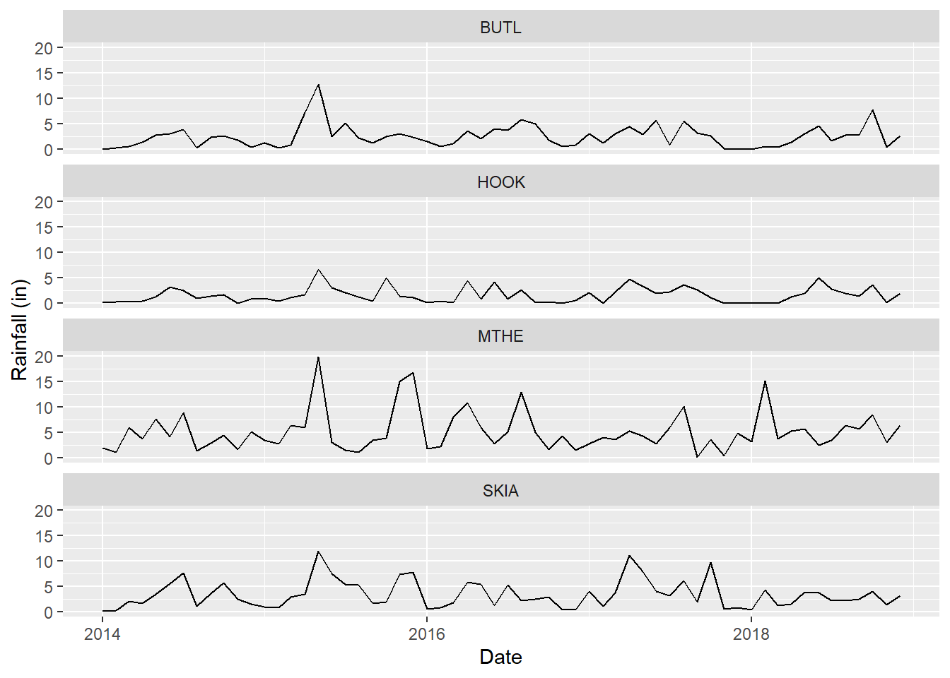
FIGURE 3.1: Faceted line graph of monthly rainfall generated with the mesomnth dataset.
3.2.1 Counts
When summarizing data, it is often necessary to count the number of values used. This can be accomplished with the dplyr function n(), which will include NA values in the count, or sum(!is.na(x)) which will exclude them. It’s a good idea to count data when summarizing them to see the sample sizes that are being used to calculate the summary statistics for each group.
This example uses the mesonew data from the previous section. The data frame is first grouped by location, year, and month. Several summary variables are then calculated with summarize(). The new n_rows column is a count of all observations for each group. The obs_hmax column is a count of the number of rows that do not have missing data for maximum humidity. The pv_hmax column is calculated as the percentage of observations that have valid maximum humidity data for each group. The mutate() function is used to add a date column to the mesomissing data frame.
mesomissing <- mesonew %>%
  group_by(STID, YEAR, MONTH) %>%
  summarize(n_rows = n(),
            obs_hmax = sum(!is.na(HMAX)),
            pv_hmax = 100 * obs_hmax/n_rows) %>%
  mutate(DATE = as.Date(paste(YEAR, MONTH, "1", sep = "-")))
glimpse(mesomissing)
## Rows: 240
## Columns: 7
## Groups: STID, YEAR [20]
## $ STID     <chr> "BUTL", "BUTL", "BUTL", "BUTL", "BUTL", "…
## $ YEAR     <dbl> 2014, 2014, 2014, 2014, 2014, 2014, 2014,…
## $ MONTH    <dbl> 1, 2, 3, 4, 5, 6, 7, 8, 9, 10, 11, 12, 1,…
## $ n_rows   <int> 31, 28, 31, 30, 31, 30, 31, 31, 30, 31, 3…
## $ obs_hmax <int> 31, 28, 31, 30, 31, 30, 31, 31, 30, 31, 3…
## $ pv_hmax  <dbl> 100, 100, 100, 100, 100, 100, 100, 100, 1…
## $ DATE     <date> 2014-01-01, 2014-02-01, 2014-03-01, 2014…
The resulting data frame contains information about when and where there are missing data. An efficient way to explore these data is using a simple plot. The following example generates a line plot, similar to the examples in Chapter 2, that displays the monthly time series of missing data using a separate plot for each site (Figure 3.2).
ggplot(data = mesomissing) +
  geom_line(mapping = aes(x = DATE, y = pv_hmax)) +
  facet_wrap(~ STID, ncol = 1) +
  labs(x = "Date",
       y = "% Valid Max Humidity Observations",
       color = "Station ID")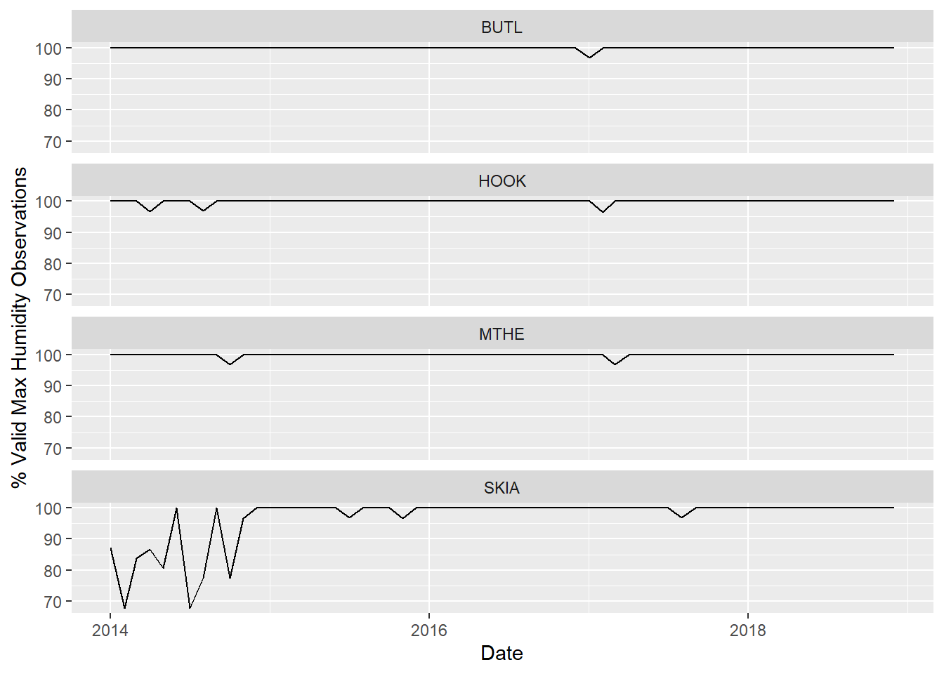
FIGURE 3.2: Line graphs of valid humidity observations for four stations.
3.2.2 Summary Functions
Up to this point, only a few summary functions have been covered: sum(), mean(), and n(). Many other summary functions are available including:
- Measures of central tendency, including the
median()as well as themean(). - Measure of variability, including
sd(), the standard deviation;IQR(), the inter-quartile range; andmad(), the mean absolute deviation. - Measures of rank, including
min(), the minimum value;quantile(), the data value associated with a given percentile; andmax(), the maximum value. - Counts, including
n(), which counts all rows; andn_distinct(), which counts the number of unique values.
3.3 Pivoting Data
Almost all of the data used in environmental geography applications can be stored and manipulated in data frames, but the format of the data frame can differ. Consider the Mesonet data where each observation is indexed by a location (station) and a time (month and year). Each weather variable, such as rainfall, is stored in a separate column. The rainfall at a particular location and time can be determined by referencing the appropriate row based on the values in the station, month, and year columns. This is what is called a “long” format, which minimizes the number of columns by increasing the number of rows in the dataset.
These data could also be stored in a “wide” format. For example, rainfall data from each station could be stored as a separate column with one row for each combination of month and year. The rainfall at a particular location and time would then be determined by referencing the appropriate column for a given station and the appropriate row based on values in the month and year columns.
In general, the “long” format is considered to be a more efficient and “tidy” way to format and process data. This idea of “tidy” data is the conceptual foundation for the tidyr package as well as the larger tidyverse collection of packages. In most cases, a long data format with fewer columns and more rows is easiest to manipulate using dplyr functions and is the format needed for plotting with ggplot() and running many types of statistical models. However, there are other situations where a wider format can be more suitable for data manipulation and analysis. Therefore the tidyr package provides two important functions called pivot_longer() and pivot wider() that can be used to reformat data frames.
Consider the problem of plotting both minimum and maximum temperatures on the same graph with ggplot(). In the current mesomnth data frame, they are in separate columns - TMIN and TMAX. To plot them in the same graph with different aesthetics, it is helpful to have all of the temperature observations in a single values column and to have a second names column that indicates the type of temperature measurement (minimum or maximum). The pivot_longer() function takes three basic arguments. The cols argument specifies which columns from the input dataset will be combined into the new values column. The one_of() function is used to specify multiple column names from the input data frame. The values_to argument specifies the name of the new column that will hold the data values. The names_to argument specifies the column with the new variable names. The mutate() function is also used to convert tstat from a character variable to a labeled factor.
temp_tidy <- mesomnth %>%
  pivot_longer(cols = one_of("TMAX", "TMIN"),
               values_to = "temp",
               names_to = "tstat") %>%
  mutate(tstat = factor(tstat,
                        levels = c("TMAX", "TMIN"),
                        labels = c("Maximum", "Minimum")))
glimpse(temp_tidy)
## Rows: 480
## Columns: 9
## Groups: STID, YEAR [20]
## $ STID  <chr> "BUTL", "BUTL", "BUTL", "BUTL", "BUTL", "BUT…
## $ YEAR  <dbl> 2014, 2014, 2014, 2014, 2014, 2014, 2014, 20…
## $ MONTH <dbl> 1, 1, 2, 2, 3, 3, 4, 4, 5, 5, 6, 6, 7, 7, 8,…
## $ HMAX  <dbl> 76.27871, 76.27871, 88.79679, 88.79679, 79.4…
## $ HMIN  <dbl> 27.18097, 27.18097, 41.16464, 41.16464, 27.0…
## $ RAIN  <dbl> 0.01, 0.01, 0.26, 0.26, 0.59, 0.59, 1.33, 1.…
## $ DATE  <date> 2014-01-01, 2014-01-01, 2014-02-01, 2014-02…
## $ tstat <fct> Maximum, Minimum, Maximum, Minimum, Maximum,…
## $ temp  <dbl> 52.02516, 21.58161, 47.52321, 22.25393, 61.0…
Now there is only a single column with temperature measurements (temp), and another column with a code that indicates the type of temperature measurement (tstat). However, the temp_tidy data frame has twice as many rows as the original mesomnth data frame because each minimum and maximum temperature value occupies a separate row. The tstat column is now a factor, and printing the data frame with glimpse() shows the more interpretable class labels (Maximum and Minimum) instead of the original variable codes (TMAX and TMIN).
Organizing the data in this long format makes it easier to generate a graph with ggplot() that includes minimum and maximum temperatures (Figure 3.3). The labels of the tstat factor are shown in the legend, and the legend title is modified using the labs() function.
ggplot(temp_tidy) +
  geom_line(aes(x = DATE,
                y = temp,
                color = tstat)) +
  facet_wrap(facets = vars(STID),
             ncol = 1,
             scales = "free_y") +
  labs(color = "Temperature",
       x = "Date",
y = "Temperature (\u00B0F)") 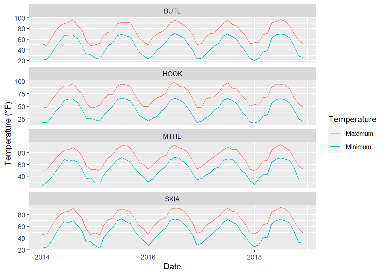
FIGURE 3.3: Line graph of monthly minimum and maximum temperatures at four stations.
When observations are distributed across multiple rows, it is sometimes necessary to reorganize the data into a wide format with multiple columns. For example, consider the problem of generating a table with just one row for each location and columns containing the total rainfall for each month in 2018. The code below shows how to accomplish this task using several dplyr functions. The data are filtered to include only records from 2018, the necessary columns are selected, missing data codes are replaced by NA, and total rainfall is calculated for each month at each weather station. The tidyr pivot_wider() function is then used to create a separate column for each monthly rainfall summary. The values_from argument indicates the input column with data to be distributed over multiple output columns. The names of these new columns will be generated by pasting the names_prefix string to the values in the names_from column.
meso2018 <- mesobig %>%
  filter(YEAR == 2018) %>%
  select(STID, MONTH, RAIN) %>%
  mutate(RAIN = replace(RAIN, RAIN <= -990 | RAIN >= 990, NA)) %>%
  group_by(STID, MONTH) %>%
  summarise(RAIN = sum(RAIN, na.rm=T)) %>%
  pivot_wider(values_from = RAIN,
              names_from = MONTH,
              names_prefix = "M")
The meso2018 data frame now has only 2018 data with one row for each station. Twelve columns named M1-M12 contain the monthly rainfall observations from January through December.
glimpse(meso2018)
## Rows: 142
## Columns: 13
## Groups: STID [142]
## $ STID <chr> "ACME", "ADAX", "ALTU", "ALV2", "ALVA", "ANT2…
## $ M1   <dbl> 0.13, 0.37, 0.01, 0.00, 0.00, 1.33, 0.00, 0.1…
## $ M2   <dbl> 2.12, 7.50, 0.79, 0.34, 0.00, 10.31, 0.00, 2.…
## $ M3   <dbl> 0.67, 3.91, 0.54, 1.58, 0.00, 2.67, 0.00, 0.7…
## $ M4   <dbl> 1.80, 2.97, 0.97, 1.55, 0.00, 2.93, 0.00, 1.2…
## $ M5   <dbl> 4.77, 4.20, 3.62, 9.17, 0.00, 3.56, 0.00, 4.3…
## $ M6   <dbl> 4.25, 4.81, 2.24, 4.32, 0.00, 4.70, 0.00, 4.3…
## $ M7   <dbl> 3.04, 2.36, 1.31, 3.25, 0.00, 2.99, 0.00, 2.0…
## $ M8   <dbl> 1.71, 7.11, 7.05, 4.08, 0.00, 5.93, 0.00, 1.1…
## $ M9   <dbl> 10.19, 11.37, 3.51, 4.72, 0.00, 6.30, 0.00, 7…
## $ M10  <dbl> 6.61, 7.42, 8.60, 8.18, 0.00, 7.48, 0.00, 5.5…
## $ M11  <dbl> 0.54, 0.40, 0.24, 0.41, 0.00, 1.90, 0.00, 0.4…
## $ M12  <dbl> 5.44, 5.92, 1.09, 2.58, 0.00, 7.65, 0.00, 3.5…
3.4 Joining Tables
Table joins are a concept shared across many data science disciplines and are implemented in relational database management systems such as MySQL. With a join, two tables are connected to each other through variables called keys, which are columns found in both tables. For the Mesonet data, possible key columns include STID, YEAR, or MONTH.
To map the mesonet summaries, we will need to add information about the geographic coordinates of each station to the summary table. This information is in a separate dataset that contains, among other variables, the station ID codes and the latitude and longitude of each weather station. There are several join functions available in dplyr. All of these functions take tables as arguments, which we will call x and y for simplicity. However, each function operates a bit differently.
inner_join(): returns all rows from x that have matching key variables in y, and all columns from x and y. If there are multiple matches between x and y, all combinations of the matches are returned.left_join(): returns all rows from x, and all columns from x and y. Rows in x with matching key variables in y will contain data in the y columns, and rows with no match in y will have NA values in the y columns. If there are multiple matches between x and y, all combinations of the matches are returned.right_join(): returns all rows from y, and all columns from x and y. Rows in y with matching key variables in x will contain data in the x columns, and rows with no match in x will have NA values in the x columns. If there are multiple matches between x and y, all combinations of the matches are returned.full_join(): returns all rows and all columns from both x and y. Where there are no matching values, the function returnsNAfor columns in the unmatched table.
In this example, the inner_join() function is used to join the geographic coordinates to the existing meso2018 table. Both datasets have a station ID column, but the column name is in upper case in meso2018 and in lower case in geo_coords. Specifying the by argument as c("STID" = "stid") indicates that these are the key columns that need to be matched from the x and y tables. In the call to inner_join(), the x table is the meso2018 data frame that comes through the pipe, and the y table is the geo_coords data frame specified as the first function argument.
geo_coords <- read_csv("geoinfo.csv", show_col_types = FALSE)
mesospatial <- meso2018 %>%
  inner_join(geo_coords, by = c("STID" = "stid"))
mesospatial
## # A tibble: 142 × 24
## # Groups:   STID [142]
##    STID     M1    M2    M3    M4    M5    M6    M7    M8
##    <chr> <dbl> <dbl> <dbl> <dbl> <dbl> <dbl> <dbl> <dbl>
##  1 ACME   0.13  2.12  0.67  1.8   4.77  4.25  3.04  1.71
##  2 ADAX   0.37  7.5   3.91  2.97  4.2   4.81  2.36  7.11
##  3 ALTU   0.01  0.79  0.54  0.97  3.62  2.24  1.31  7.05
##  4 ALV2   0     0.34  1.58  1.55  9.17  4.32  3.25  4.08
##  5 ALVA   0     0     0     0     0     0     0     0
##  6 ANT2   1.33 10.3   2.67  2.93  3.56  4.7   2.99  5.93
##  7 ANTL   0     0     0     0     0     0     0     0
##  8 APAC   0.19  2.21  0.71  1.28  4.32  4.38  2     1.14
##  9 ARD2   0.12  7.31  2.36  1.93  6.84  1.45  0.9   4.26
## 10 ARDM   0     0     0     0     0     0     0     0
## # … with 132 more rows, and 15 more variables: M9 <dbl>,
## #   M10 <dbl>, M11 <dbl>, M12 <dbl>, stnm <dbl>,
## #   name <chr>, city <chr>, rang <dbl>, cdir <chr>,
## #   cnty <chr>, lat <dbl>, lon <dbl>, elev <dbl>,
## #   cdiv <chr>, clas <chr>
The mesospatial data frame now contains monthly rainfall summaries and geographic coordinates for each Mesonet station, so ggplot() can be used to generate a simple map of January rainfall by plotting points with the longitudes on the x-axis, latitudes on the y-axis, and sizes scaled by January rainfall (Figure 3.4). Chapter 5 will build upon this simple example and introduce new object classes and functions for manipulating and mapping geospatial data.
ggplot(data = mesospatial) +
  geom_point(aes(x = lon,
                 y = lat,
                 size = M1),
             color = "black") +
  scale_size_continuous(name="Rainfall (mm)") +
  coord_equal() +
  labs(title="Jan 2018 Rainfall in Oklahoma") +
  theme_bw()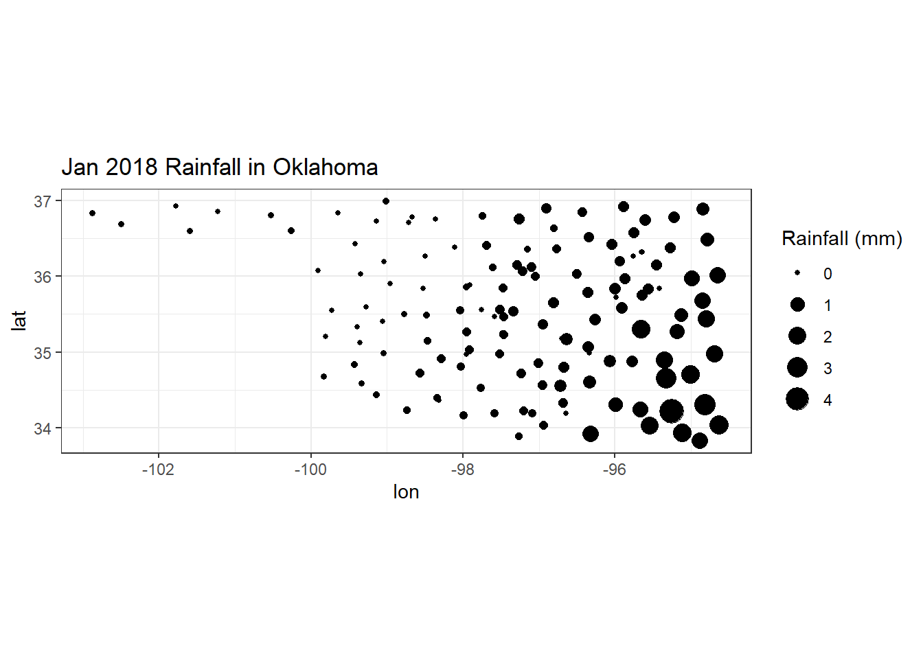
FIGURE 3.4: Graduated symbol map of January 2018 rainfall in Oklahoma.
There are many helpful resources that can help expand your knowledge of dplyr, tidyr, and other tidyverse packages. Wickham and Grolemund’s R For Data Science (Wickham and Grolemund 2016) provides a comprehensive introduction to tabular data processing, visualization, and analysis. The website at https://www.tidyverse.org/ has helpful reference guides for all of the tidyverse packages. The “cheatsheets” available for dplyr and tidyr at https://www.rstudio.com/resources/cheatsheets/ are useful quick reference guides.
3.5 Practice
Write code to filter the rows from the Skiatook station (SKIA) where the precipitation is greater than one inch using the
mesosmdataset.Write code to select only the month, year, station ID, and rainfall columns using the
mesosmdataset.Write code to create a new column to the
mesosmdataset called RAINMM that contains the rainfall values converted from inches to millimeters (1 mm = 0.3937 in).Use the
mesobigdataset to determine the percent of valid rainfall observations for each combination of station, month, and year and generate a graph of the results.Use the
mesosmdataset to generate a data frame containing minimum and maximum humidity in long format and graph the results.