CHAPTER 5 Analysis of Variance
Because of the assumption of normality of the error terms, we can now do inferences in regression analysis. In particular, one of our interest is in doing an analysis of variance. This will help us assess whether we attained our aim in modeling: to explain the variation in \(Y\) in terms of the \(X\)s.
Definition 5.1 In analysis of variance (ANOVA), the total variation displayed by a set of observations, as measured by the sum of squares of deviations from the mean, are separated into components associated with defined sources of variation used as criteria of classification for observations.
Remarks:
An ANOVA decomposes the variation in \(Y\) into those that can be explained by the model and the unexplained portion.
There is variation in \(\textbf{Y}\) as in all statistical data. If all \(Y_i\)s were identically equal, in which case, \(Y_i = \bar{Y}\) for all \(i\), there would be no statistical problems (but not realistic!).
The variation of the \(Y_i\) is conventionally measured in terms of \(Y_i − \bar{Y}\).
5.1 ANOVA Table and F-test for Regression Relation
This section makes use of concepts in Sum of Squares and Mean Squares. Make sure to review them first.
GOAL: In this section, we will show a test for the hypotheses:
\[ Ho: \beta_1=\beta_2,...,\beta_k=0 \quad \text{vs}\quad Ha:\text{at least one }\beta_j\neq0 \text{ for } j=1,2,...,k \]
We want to test if fitting a line on the data is worthwhile.
| Source of Variation | df | Sum of Squares | Mean Square | F-stat | p-value |
|---|---|---|---|---|---|
| Regression | \(p-1\) | \(SSR\) | \(MSR\) | \(F_c=\frac{MSR}{MSE}\) | \(P(F>F_c)\) |
| Error | \(n-p\) | \(SSE\) | \(MSE\) | ||
| Total | \(n-1\) | \(SST\) |
The ANOVA table is a classical result that is always presented in regression analysis.
It is a table of results that details the information we can extract from doing the F-test for Regression Relation (oftentimes simply referred to as the F-test for ANOVA).
The said test has the following competing hypotheses:
\[ Ho: \beta_1=\beta_2,...,\beta_k=0 \quad vs\quad Ha:\text{at least one }\beta_j\neq0 \text{ for } j=1,2,...,k \]
It basically tests whether it is still worthwhile to do regression on the data.
Definition 5.2 (F-test for Regression Relation)
For testing \(Ho: \beta_1=\beta_2,...,\beta_k=0\) vs \(Ha:\text{at least one }\beta_j\neq0 \text{ for } j=1,2,...,k\), the test statistic is
\[ F_c=\frac{MSR}{MSE}=\frac{SSR/(p-1)}{SSE/(n-p)}\sim F_{(p-1),(n-p)},\quad \text{under } Ho \]
The critical region of the test is \(F_c>F^\alpha_{(p-1),(n-p)}\)
Remarks:
The distribution of the statistic \(F_c\) was derived from Exercise 4.8
When null is rejected, possible interpretation is
“there is at least one independent variable that has a unique linear contribution to the variation of the dependent variable”.
A significant F-test implies at least one predictor is useful, but does not tell which one. You should follow-up with:
partial F-tests for individual predictors (Testing that one slope parameter is 0) or
t-tests (Hypothesis Testing for Individual Slope Parameters)
More details about this test in Testing that all of the slope parameters are 0
Example in R
We use the data by F.J. Anscombe again which contains U.S. State Public-School Expenditures in 1970.
| education | income | young | urban | |
|---|---|---|---|---|
| ME | 189 | 2824 | 350.7 | 508 |
| NH | 169 | 3259 | 345.9 | 564 |
| VT | 230 | 3072 | 348.5 | 322 |
| MA | 168 | 3835 | 335.3 | 846 |
| RI | 180 | 3549 | 327.1 | 871 |
| CT | 193 | 4256 | 341.0 | 774 |
| NY | 261 | 4151 | 326.2 | 856 |
| NJ | 214 | 3954 | 333.5 | 889 |
| PA | 201 | 3419 | 326.2 | 715 |
| OH | 172 | 3509 | 354.5 | 753 |
| IN | 194 | 3412 | 359.3 | 649 |
| IL | 189 | 3981 | 348.9 | 830 |
| MI | 233 | 3675 | 369.2 | 738 |
| WI | 209 | 3363 | 360.7 | 659 |
| MN | 262 | 3341 | 365.4 | 664 |
| IO | 234 | 3265 | 343.8 | 572 |
| MO | 177 | 3257 | 336.1 | 701 |
| ND | 177 | 2730 | 369.1 | 443 |
| SD | 187 | 2876 | 368.7 | 446 |
| NE | 148 | 3239 | 349.9 | 615 |
| KA | 196 | 3303 | 339.9 | 661 |
| DE | 248 | 3795 | 375.9 | 722 |
| MD | 247 | 3742 | 364.1 | 766 |
| DC | 246 | 4425 | 352.1 | 1000 |
| VA | 180 | 3068 | 353.0 | 631 |
| WV | 149 | 2470 | 328.8 | 390 |
| NC | 155 | 2664 | 354.1 | 450 |
| SC | 149 | 2380 | 376.7 | 476 |
| GA | 156 | 2781 | 370.6 | 603 |
| FL | 191 | 3191 | 336.0 | 805 |
| KY | 140 | 2645 | 349.3 | 523 |
| TN | 137 | 2579 | 342.8 | 588 |
| AL | 112 | 2337 | 362.2 | 584 |
| MS | 130 | 2081 | 385.2 | 445 |
| AR | 134 | 2322 | 351.9 | 500 |
| LA | 162 | 2634 | 389.6 | 661 |
| OK | 135 | 2880 | 329.8 | 680 |
| TX | 155 | 3029 | 369.4 | 797 |
| MT | 238 | 2942 | 368.9 | 534 |
| ID | 170 | 2668 | 367.7 | 541 |
| WY | 238 | 3190 | 365.6 | 605 |
| CO | 192 | 3340 | 358.1 | 785 |
| NM | 227 | 2651 | 421.5 | 698 |
| AZ | 207 | 3027 | 387.5 | 796 |
| UT | 201 | 2790 | 412.4 | 804 |
| NV | 225 | 3957 | 385.1 | 809 |
| WA | 215 | 3688 | 341.3 | 726 |
| OR | 233 | 3317 | 332.7 | 671 |
| CA | 273 | 3968 | 348.4 | 909 |
| AK | 372 | 4146 | 439.7 | 484 |
| HI | 212 | 3513 | 382.9 | 831 |
Our dependent variable is the Per-capita income in dollars
##
## Call:
## lm(formula = income ~ education + young + urban, data = Anscombe)
##
## Residuals:
##     Min      1Q  Median      3Q     Max
## -438.54 -145.21  -41.65  119.20  739.69
##
## Coefficients:
##              Estimate Std. Error t value Pr(>|t|)
## (Intercept) 3011.4633   609.4769   4.941 1.03e-05 ***
## education      7.6313     0.8798   8.674 2.56e-11 ***
## young         -6.8544     1.6617  -4.125  0.00015 ***
## urban          1.7692     0.2591   6.828 1.49e-08 ***
## ---
## Signif. codes:  0 '***' 0.001 '**' 0.01 '*' 0.05 '.' 0.1 ' ' 1
##
## Residual standard error: 259.7 on 47 degrees of freedom
## Multiple R-squared:  0.7979, Adjusted R-squared:  0.785
## F-statistic: 61.86 on 3 and 47 DF,  p-value: 2.384e-16
The F-statistic and the p-value are already shown using the summary() function.
At this point, the ANOVA table is not necessary anymore since result of the F-test is already presented.
For the sake of this example, how do we output the ANOVA table?
## Analysis of Variance Table
##
## Response: income
##           Df  Sum Sq Mean Sq F value    Pr(>F)
## education  1 6988589 6988589 103.658 1.788e-13 ***
## young      1 2381325 2381325  35.321 3.281e-07 ***
## urban      1 3142811 3142811  46.616 1.493e-08 ***
## Residuals 47 3168730   67420
## ---
## Signif. codes:  0 '***' 0.001 '**' 0.01 '*' 0.05 '.' 0.1 ' ' 1
Unfortunately, the output of anova() in R does not directly provide the SST, SSR, and SSE, and the F test of the full model. That is, only Sequential F-tests are presented. See more about this in [Testing a slope parameter equal to 0 sequentially]
In this example, we can just try to calculate the important figures manually.
Y    <- Anscombe$income
Ybar <- mean(Anscombe$income)
Yhat <- fitted(mod_anscombe)

SST  <- sum((  Y  - Ybar)^2)  # Total Sum of Squares
SSR  <- sum((Yhat - Ybar)^2)  # Regression Sum of Squares
SSE  <- sum((Yhat -   Y )^2)  # Error Sum of Squares

n    <- nrow(Anscombe)
p    <- length(coefficients(mod_anscombe))

MSR  <- SSR/(p-1)
MSE  <- SSE/(n-p)

F_c  <- MSR/MSE
Pr_F <- pf(F_c,p-1,n-p, lower.tail = F)| Source | df | Sum_of_Squares | Mean_Square | F_value | Pr_F |
|---|---|---|---|---|---|
| Regression | 3 | 12512724.9115 | 4170908.3038 | 61.8648 | <0.0001 |
| Error | 47 | 3168729.6767 | 67419.7804 | ||
| Total | 50 | 15681454.5882 |
At 0.05 level of significance, there is sufficient evidence to conclude that there is at least one \(\beta_j\neq0\).
5.2 The General Linear Test
We are already done with the estimation of the model parameters (mostly based on Least Squares).
As a way to verify whether it is worthwhile to keep variables in our model, we can do hypothesis tests on the model parameters.
GOAL: Compare 2 models, reduced model vs full model
We want to know if adding more independent variables improves a linear model.
For the multiple linear regression model, these are some hypotheses that we may want to test.
Testing that all of the slope parameters are 0
\(Ho: \beta_1 = \beta_2 = \cdots = \beta_k = 0\)
\(Ha: \text{at least one }\beta_j \neq 0 \quad \text{for all }\ j = 1, 2,..., k\)
Testing that one slope parameter is 0
- \(Ho: \beta_j = 0\)
- \(Ha: \beta_j \neq 0\)
Testing several slope parameters equal to 0
\(Ho: \beta_j \text{ are all equal to 0} \text{ for some } j \in {1,...,k}\)
\(Ha: \text{at least one } \beta_j \neq 0 \text{ for some } j \in {1,...,k}\)
All of these hypotheses about regression coefficients can actually be tested using a unified approach!
Before the discussion of the actual tests, some important definitions and results will be presented as preliminaries.
Full and Reduced Models
Definition 5.3 (Full Model and Reduced Model)
- The full model or unrestricted model is the model containing all the independent variables that are or interest.
- The reduced model or restricted model is the model when the null hypothesis holds.
Example
Let’s use again the Anscombe dataset with the following variables:
y:incomex1:educationx2:youngx3:urban
The full model includes all the predictor variables. \[ y=\beta_0+\beta_1x_1+\beta_2x_2+\beta_3x_3+\varepsilon \]
# Fit the full model
full_model <- lm(income ~ education + young + urban, data = Anscombe)

# Summary of the full model
summary(full_model)
##
## Call:
## lm(formula = income ~ education + young + urban, data = Anscombe)
##
## Residuals:
## Min 1Q Median 3Q Max
## -438.54 -145.21 -41.65 119.20 739.69
##
## Coefficients:
## Estimate Std. Error t value Pr(>|t|)
## (Intercept) 3011.4633 609.4769 4.941 1.03e-05 ***
## education 7.6313 0.8798 8.674 2.56e-11 ***
## young -6.8544 1.6617 -4.125 0.00015 ***
## urban 1.7692 0.2591 6.828 1.49e-08 ***
## ---
## Signif. codes: 0 '***' 0.001 '**' 0.01 '*' 0.05 '.' 0.1 ' ' 1
##
## Residual standard error: 259.7 on 47 degrees of freedom
## Multiple R-squared: 0.7979, Adjusted R-squared: 0.785
## F-statistic: 61.86 on 3 and 47 DF, p-value: 2.384e-16The reduced model includes only a subset of the predictor variables.
For example, excluding x3 by assuming \(\beta_3=0\) (null is true). \[
y=\beta_0+\beta_1x_1+\beta_2x_2+\varepsilon
\]
# Fit the reduced model
reduced_model <- lm(income ~ education + young, data = Anscombe)
# Summary of the reduced model
summary(reduced_model)##
## Call:
## lm(formula = income ~ education + young, data = Anscombe)
##
## Residuals:
## Min 1Q Median 3Q Max
## -590.04 -220.72 -26.48 186.13 891.03
##
## Coefficients:
## Estimate Std. Error t value Pr(>|t|)
## (Intercept) 4783.061 770.168 6.210 1.20e-07 ***
## education 9.588 1.162 8.253 9.15e-11 ***
## young -9.585 2.252 -4.256 9.61e-05 ***
## ---
## Signif. codes: 0 '***' 0.001 '**' 0.01 '*' 0.05 '.' 0.1 ' ' 1
##
## Residual standard error: 362.6 on 48 degrees of freedom
## Multiple R-squared: 0.5975, Adjusted R-squared: 0.5807
## F-statistic: 35.63 on 2 and 48 DF, p-value: 3.266e-10Decomposition of SSR into Extra Sum of Squares
In regression work, the question often arises as to whether or not it is worthwhile to include certain terms in the model. This question can be investigated by considering the extra portion of the regression sum of squares which arises due to the fact that the terms under consideration were in the model.
Definition 5.4 (Extra Sum of Squares)
Extra Sums of Squares (or Sequential Sum of Squares) represents the difference in Regression Sums of Squares (SSR) between two models.
\[
ESS = SSR(F)-SSR(R)
\]
where \(SSR(F)\) is the SSR of the full model and \(SSR(R)\) is the SSR of the reduced model.
Remarks:
The extra sum of squares reflect the increase in the regression sum of squares achieved by introducing the new variable.
\(SSR(R) + ESS = SSR(F)\)
Suppose you have two variables \(X_1\) and \(X_2\) being considered in the model. The increase in regression sum of squares when \(X_2\) is added given that \(X_1\) was already in the model may be denoted by \(SSR(X_2|X_1)=SSR(X_1,X_2)-SSR(X_1)\)
Also, since always \(SST = SSR + SSE\) , and SST of the full model and the reduced model are the same:
\[\begin{align} SSR(X_2|X_1)&=SSR(X_1,X_2)-SSR(X_1)\\ &=(SST-SSE(X_1,X_2))-(SST-SSE(X_1))\\ &=SSE(X_1)-SSE(X_1,X_2)\\ \end{align}\]Extensions for 3 or more independent variables are straightforward.
ESS can also be thought of as the marginal decrease in SSE when an additional set of predictors is incorporated into the model, given that another independent variable is already in the model.
The SSE of the full model is always less than or equal the SSE of the reduced model: \(SSE(F ) \leq SSE(R)\)
More predictors \(\rightarrow\) Better Fit \(\rightarrow\) smaller deviations around the fitted regression line
General Linear Test
Definition 5.5 (General Linear Test)
The General Linear Test is used to determine if adding a variable/s will help improve the model fit. This is done by comparing a smaller (reduced) model with fewer variables vs a larger (full) model with added variables. We use an F-statistic to decide whether or not to reject the smaller reduced model in favor of the larger full model.
The basic steps of the general linear test are
Fit the full model and obtain the error sum of squares \(SSE(F)\)
Fit the reduced model and obtain the error sum of squares \(SSE(R)\)
The test statistic will be \[ F^*=\frac{\left(\frac{SSE(R)-SSE(F)}{\text{df}_R-\text{df}_F}\right)}{\frac{SSE(F)}{\text{df}_F}} \] and the critical region is \(F^*>F_{(\alpha,\text{df}_R-\text{df}_F,\text{df}_F)}\)
Remarks:
- (Almost equal SSE of reduced vs full)
- If \(SSE(F)\) is not much less than \(SSE(R)\), using the full model (or having additional independent variable/s) does not account for much more of the variability of \(Y_i\) than the reduced model.
- This means that the data suggest that the null hypothesis holds.
- If the additional independent variable does not contribute much to the model, then it is better to use the reduced model than the full model to achieve parsimony.
- (Large SSE of reduced vs full)
- On the other hand, a large difference \(SSE(R) − SSE(F)\) suggests that the alternative hypothesis holds because the addition of parameters in the model helps to reduce substantially the variation of the observations \(Y_i\) around the fitted regression line.
- The numerator of the general linear F-statistic is the extra sum of squares between the full model and the reduced model.
We will use the general linear test for constructing tests for different hypotheses.
The overarching goal of the following sections is to determine if “adding” a variable improves the model model fit.
We will use the General Linear Test in the following examples.
Concepts such as the Partial F test and Sequential F test will be introduced.
Examples in R are also presented, using the Anscombe dataset.
Let
\(Y_{i}\) =
income: per-capita income (in dollars) of state \(i\)\(X_{i1}\) =
education: per-capita education expenditure (in dollars) of state \(i\)\(X_{i2}\) =
young: proportion under 18 (per 1000) of state \(i\)\(X_{i3}\) =
urban: Proportion urban (per 1000) of state \(i\)
Testing that all of the slope parameters are 0
Suppose we are testing whether all parameters equal to 0
- \(Ho:\beta_1=\beta_2=\cdots=\beta_k=0\)
- \(Ha:\) at least one \(\beta_j\neq0\) for \(j=1,\cdots,k\)
Using the General Linear Test,
- The \(SSE(F)\) is just the usual error sum of squares seen in the ANOVA table.
- Since the null is \(\beta_j\) are all equal to 0, the reduced model suggests that none of the variations in the response Y is explained by any of the predictors. Therefore, \(SSE(R)\) is just the total sum of squares, which is the \(SST\) that appears in the ANOVA table.
With this, the F Statistic is \[\begin{align} F^*&=\frac{\left(\frac{SSE(R)-SSE(F)}{\text{df}_R-\text{df}_F}\right)}{\frac{SSE(F)}{\text{df}_F}}\\ &=\frac{\left(\frac{SST-SSE}{(n-1)-(n-p)}\right)}{\frac{SSE}{n-p}}\\ &=\frac{SSR/(p-1)}{SSE/(n-p)} \end{align}\]
and the critical region to reject \(Ho\) is \(F^*>F_{(\alpha,p-1,n-p)}\)
This is just the usual F-test for regression Relation!
We already saw this in [ANOVA Table and F Test for Regression Relation].
Illustration in R:
The full model includes all variables, while the reduced model only includes the intercept.
- Full Model: \(Y_i=\beta_0+\beta_1X_{i1} + \beta_2 X_{i2} + \beta_3 X_{i3}+\varepsilon_i\)
- Reduced Model: \(Y_i=\beta_0+\varepsilon_i\)
The hypotheses can be set as: - \(Ho:\beta_1=\beta_2=\beta_3=0\) - \(Ha:\beta_1\neq0 \text{ or } \beta_2\neq 0\text{ or } \beta_3\neq 0\)
We use the anova() function to compare the full model vs the reduced model.
# Full Model: all variables included
F_model <- lm(income~education+young+urban, data = Anscombe)
# Reduced Model: no variables included, all beta_j = 0
R_model <- lm(income~1, data = Anscombe)
# Performing the F-test: reduced vs full
anova(R_model, F_model)## Analysis of Variance Table
##
## Model 1: income ~ 1
## Model 2: income ~ education + young + urban
## Res.Df RSS Df Sum of Sq F Pr(>F)
## 1 50 15681455
## 2 47 3168730 3 12512725 61.865 2.384e-16 ***
## ---
## Signif. codes: 0 '***' 0.001 '**' 0.01 '*' 0.05 '.' 0.1 ' ' 1In this output,
\(\text{df of }SSE(R) = 51 - 1 = 50\)
\(\text{df of }SSE(F) = 51 - 4 = 47\)
Conclusion: At 0.05 level of significance, there is sufficient evidence to conclude that there is at least one slope parameter that is not equal to 0. That is, from the 3 variables, at least one variable contributes to the model.
Note: The F-Statistic here is the same as the F-statistic shown in the summary() output, which is 61.86
##
## Call:
## lm(formula = income ~ education + young + urban, data = Anscombe)
##
## Residuals:
##     Min      1Q  Median      3Q     Max
## -438.54 -145.21  -41.65  119.20  739.69
##
## Coefficients:
##              Estimate Std. Error t value Pr(>|t|)
## (Intercept) 3011.4633   609.4769   4.941 1.03e-05 ***
## education      7.6313     0.8798   8.674 2.56e-11 ***
## young         -6.8544     1.6617  -4.125  0.00015 ***
## urban          1.7692     0.2591   6.828 1.49e-08 ***
## ---
## Signif. codes:  0 '***' 0.001 '**' 0.01 '*' 0.05 '.' 0.1 ' ' 1
##
## Residual standard error: 259.7 on 47 degrees of freedom
## Multiple R-squared:  0.7979, Adjusted R-squared:  0.785
## F-statistic: 61.86 on 3 and 47 DF, p-value: 2.384e-16Testing that one slope parameter is 0
Suppose we are testing a slope parameter equal to 0
- \(Ho:\beta_j=0\)
- \(Ha:\) \(\beta_j\neq0\)
Using the General Linear Test,
- The \(SSE(F)\) is just the usual error sum of squares seen in the ANOVA table.
- Since the null is \(\beta_j=0\), the reduced model only removes the \(j^{th}\) variable, while keeping the rest of the independent variables. That is, \(SSE(R)=SSE(\text{w/o }X_j)\)
With this, the F Statistic is \[\begin{align} F^*&=\frac{\left(\frac{SSE(R)-SSE(F)}{\text{df}_R-\text{df}_F}\right)}{\frac{SSE(F)}{\text{df}_F}}\\ &=\frac{\left(\frac{SSE(\text{w/o } X_j)-SSE}{(n-(p-1))-(n-p)}\right)}{\frac{SSE}{n-p}}\\ &=\frac{\left(\frac{SSR(X_j|X_1,...,X_{j-1},X_{j+1},..., X_p)-SSE}{1}\right)}{\frac{SSE}{n-p}}\\ &=\frac{SSR(F)-SSR(\text{w/o } X_j)}{MSE} \end{align}\]
and the critical region to reject \(Ho\) is \(F^*>F_{(\alpha,1,n-p)}\)
This test is usually called the Partial F-test for one slope parameter
Remarks: Relationship of the Partial F-test and the T-test for one slope parameter
Another way to devise a test for each \(\beta_j\) is by using the probability distribution of the estimate \(\hat\beta_j\).
Recall Section 6.1 for the confidence interval and hypothesis test for \(\beta_j\) .
The goal of the Partial F-tests and the T-tests are the same, but the approaches are different
| Aspect | Partial F-test (removing \(X_j\)) | T-test |
|---|---|---|
| Purpose | To assess the significance of a single predictor when added to the model. | To assess the significance of an individual predictor’s coefficient. |
| Null Hypothesis \(Ho\) | The predictor being tested has no effect (\(\beta_j=0\)) | The predictor being tested has no effect (\(\beta_j=0\) ) |
| Alternative Hypothesis \(Ha\) | The predictor being tested has effect (\(\beta_j\neq0\)) | The predictor being tested has effect (\(\beta_j\neq0\)) |
| Test Statistic | F-statistic: \(F^*=\frac{SSR(F)-SSR(\text{w/o } X_j)}{MSE}\) | t-statistic: \(t_j=\frac{\hat{\beta}_j}{\widehat{se(\hat\beta_j})}\) |
| Interpretation | A significant F indicates the predictor improves the model fit. | A significant t indicates the predictor is significantly associated with the response variable. |
| When Used | When comparing nested models (full vs. reduced with one less predictor). | When evaluating each predictor individually within the same model. |
| Relationship | When only one predictor is tested, the F-statistic is the square of the t-statistic for that predictor. | The t-statistic is directly related to the F-statistic: \(F^*=t^2\) . |
Illustration in R
The full model includes all variables, while the reduced model removes one variable. In this example, we want to know if adding urban improves the model fit.
- Full Model: \(Y_i=\beta_0+\beta_1X_{i1} + \beta_2 X_{i2} + \beta_3 X_{i3}+\varepsilon_i\)
- Reduced Model: \(Y_i=\beta_0+\beta_1X_{i1} + \beta_2 X_{i2}+\varepsilon_i\)
The hypotheses can be set as: - \(Ho:\beta_3=0\) given \(\beta_1\neq0\) and \(\beta_2\neq0\)(or \(X_1\) and \(X_2\) are already in the model) - \(Ha:\beta_3\neq 0\)
# Reduced Model: removing urban only
R_model <- lm(income ~ education + young, data = Anscombe)

# Full Model: adding urban, all variables included
F_model <- lm(income~education+young+urban, data = Anscombe)

# Performing the F-test: full vs reduced with no urban
anova(R_model, F_model)
## Analysis of Variance Table
##
## Model 1: income ~ education + young
## Model 2: income ~ education + young + urban
## Res.Df RSS Df Sum of Sq F Pr(>F)
## 1 48 6311541
## 2 47 3168730 1 3142811 46.616 1.493e-08 ***
## ---
## Signif. codes: 0 '***' 0.001 '**' 0.01 '*' 0.05 '.' 0.1 ' ' 1Conclusion: Based on the result of the F-test, adding urban in the model significantly improves the model fit, vs if education and young are the only predictors in the model.
Testing several slope parameters equal to 0
Testing that a subset — more than one, but not all — of the slope parameters are 0
Suppose we are testing a slope parameter equal to 0
\(Ho:\) Some \(\beta_j\) are all equal to \(0\)
\(Ha:\) at least 1 of some \(\beta_j\neq0\)
This is almost the same as Testing that all of the slope parameters are 0, but the reduced model may contain at least one independent variable already.
As an illustrative example:
- \(Ho:\) \(\beta_2=\beta_3=0\) (\(\beta\) and \(X_1\) is already included in the model)
- \(Ha:\) at least 1 of the \(\beta_j\neq 0\)
Using the General Linear Test
- The full model still includes all the variables. That is, \(SSE(F)\) is the usual \(SSE\)
- Since the null is \(\beta_2=\beta_3=0\), the reduced model removes the variables \(X_2\) and \(X_3\), while keeping the rest of the independent variables. That is, \(SSE(R)=SSE(\text{w/o }X_2 \text{ and } X_3)\)
With this, the F Statistic is \[\begin{align} F^*&=\frac{\left(\frac{SSE(R)-SSE(F)}{\text{df}_R-\text{df}_F}\right)}{\frac{SSE(F)}{\text{df}_F}}\\ &=\frac{\left(\frac{SSE(\text{w/o } X_2 \text{ and } X_3)-SSE}{(n-(p-2))-(n-p)}\right)}{\frac{SSE}{n-p}}\\ &=\frac{\left(\frac{SSR(X_2,X_3|X_1,X_4,...,X_p)}{2}\right)}{\frac{SSE}{n-p}}\\ &=\frac{(SSR(F)-SSR(\text{w/o } X_2 \text{ and } X_3))/2}{MSE} \end{align}\]
and the critical region to reject \(Ho\) is \(F^*>F_{(\alpha,2,n-p)}\)
In this example, we only removed 2 variables. You can extend it to several variables.
This test is usually called the Partial F-test for several slope parameters
Illustration in R
The full model includes all 3 variables, while the reduced model has no variables young and urban. Only education will be retained.
# Reduced Model: education only, removing young and urban
R_model <- lm(income ~ education, data = Anscombe)

# Full Model: adding young and urban, all variables included
F_model <- lm(income~education+young+urban, data = Anscombe)

# Performing the F-test: reduced vs full
anova(R_model, F_model)
## Analysis of Variance Table
##
## Model 1: income ~ education
## Model 2: income ~ education + young + urban
## Res.Df RSS Df Sum of Sq F Pr(>F)
## 1 49 8692865
## 2 47 3168730 2 5524135 40.968 5.017e-11 ***
## ---
## Signif. codes: 0 '***' 0.001 '**' 0.01 '*' 0.05 '.' 0.1 ' ' 1SSE_R<-sum((Anscombe$income - fitted(R_model))^2)
SSE_F<-sum((Anscombe$income - fitted(F_model))^2)
((SSE_R - SSE_F)/2)/(SSE_F/47)## [1] 40.96821Conclusion: The addition of young and urban significantly improves the model fit, vs if education is the only predictor in the model.
Summary of the General Linear Tests
- Reduced model - Model under Ho; Full model - Model where all variables of concern are inside it.
- Extra sum of squares: \[ SSR(\text{new vars|old vars})= SSE(\text{old vars only})−SSE(\text{all vars})= SSE(R) - SSE(F) \]
- The test statistic for the general linear test is \[ F^*=\frac{\left(\frac{SSE(R)-SSE(F)}{\text{df}_R-\text{df}_F}\right)}{\frac{SSE(F)}{\text{df}_F}}\sim F(\text{df}_R-\text{df}_F,\text{df}_F), \quad \text{under } Ho \]
- The partial F-test can be made for all regression coefficients as though each corresponding variable were the last to enter the equation, to see the relative effects of each variable in excess of the others. Thus, the test is a useful criterion for adding or removing terms from the model for variable selection.
- When the variables are added one by one in stages to a regression equation, then we do a sequential F-test. This is just the partial F-test on the variable which entered the regression at that stage.
Question: Why is my slope parameter not significant?
- Recall: we reject \(Ho: \beta_j=0\) if \(|T|>t_{\alpha/2,n-p}\). Not rejecting \(Ho\) means we conclude that the variable \(X_j\) is not linearly associated with the dependent variable.
- Possible reasons of insignificant parameter:
- the predictor in question itself is not a good (linear) predictor of dependent variable
- n is too small (sample size is too small)
- p is too large (number of predictors is too large)
- SSE is too large (all of the predictors are really not of good quality)
- The predictors are highly correlated with one another.
Exercise 5.1 Suppose you have a dataset with 47 observations and 5 possible independent variables, \(X_1,X_2,X_3,X_4,X_5\), that you want to know if they linearly contribute to the variation of \(Y\).
Assuming that \(X_1\) and \(X_2\) are already in the model (i.e. \(\beta_1\neq0\) and \(\beta_2\neq0\)), derive a test (at \(\alpha\) level of significance) that shows if adding \(X_4\) and \(X_5\) improves the model fit.
Show:
Ho vs Ha
The reduced and full models
F-statistic, in terms of \(SSR(\cdot|\cdot)\) and \(SSE(.)\) where \(\cdot\) is a set of \(Xs\)
Critical Region (Decision Rule)
Coefficient of Partial Determination
In checking if one variable contributes to the model fit, we used the general linear test to show this.
Here, we also show a metric that quantifies the contribution of an independent variable to the model, related to the coefficient of determination.
Definition 5.6 (Coefficient of Partial Determination) A coefficient of partial determination (or partial \(R^2\)) measures the marginal contribution of one independent variable when all others are already included in the model.
\[\begin{align} R^2_{Y_j|1,2,...,j-1,j+1,...,k}&=\frac{SSR(X_j|X_1,X_2,...,X_{j-1},X_{j+1},...,X_k)}{SSE(X_1,X_2,...,X_{j-1},X_{j+1},...,X_k)} \\ &= \frac{SSE(R)-SSE(F)}{SSE(R)} \end{align}\]In the subscripts to \(R^2\), the entries to the left of the pipe show which variable is taken as the response and which variable is being added. The entries to the right show the variables already in the model.
Notes:
- The coefficient of partial determination is the marginal contribution of \(X_j\) to the reduction of variation in \(Y\) when \(X_1, X_2, ..., X_j-1, X_j+1, ..., X_k\) are already in the model
- This gives us the proportion of variation explained by \(X_j\) that cannot be explained by the other independent variables.
- The coefficient of partial determination can take on values between 0 and 1.
- The coefficient of partial correlation is the square root of the coefficient of partial determination. It follows the sign of the associated regression coefficient. It does not have as clear a meaning as the coefficient of partial determination.
Example in R
F_model <- lm(income~education + young + urban, data = Anscombe)
R_model <- lm(income~education + young, data = Anscombe)

# SSE of the full model
SSE_F <- sum((F_model$residuals)^2)
# SSE of the reduced model
SSE_R <- sum((R_model$residuals)^2)

(SSE_R - SSE_F)/SSE_R
## [1] 0.4979467urban explains 49.79 % of variation in income that education and young cannot explain.
5.3 The Lack of Fit Test
The classic lack-of-fit test require repeat observations at one or more X levels.
Definition 5.7 (Replication and Replicates) Repeated trials for the same levels of the independent variables are called replications and the resulting observations are called replicates.
Decomposing SSE
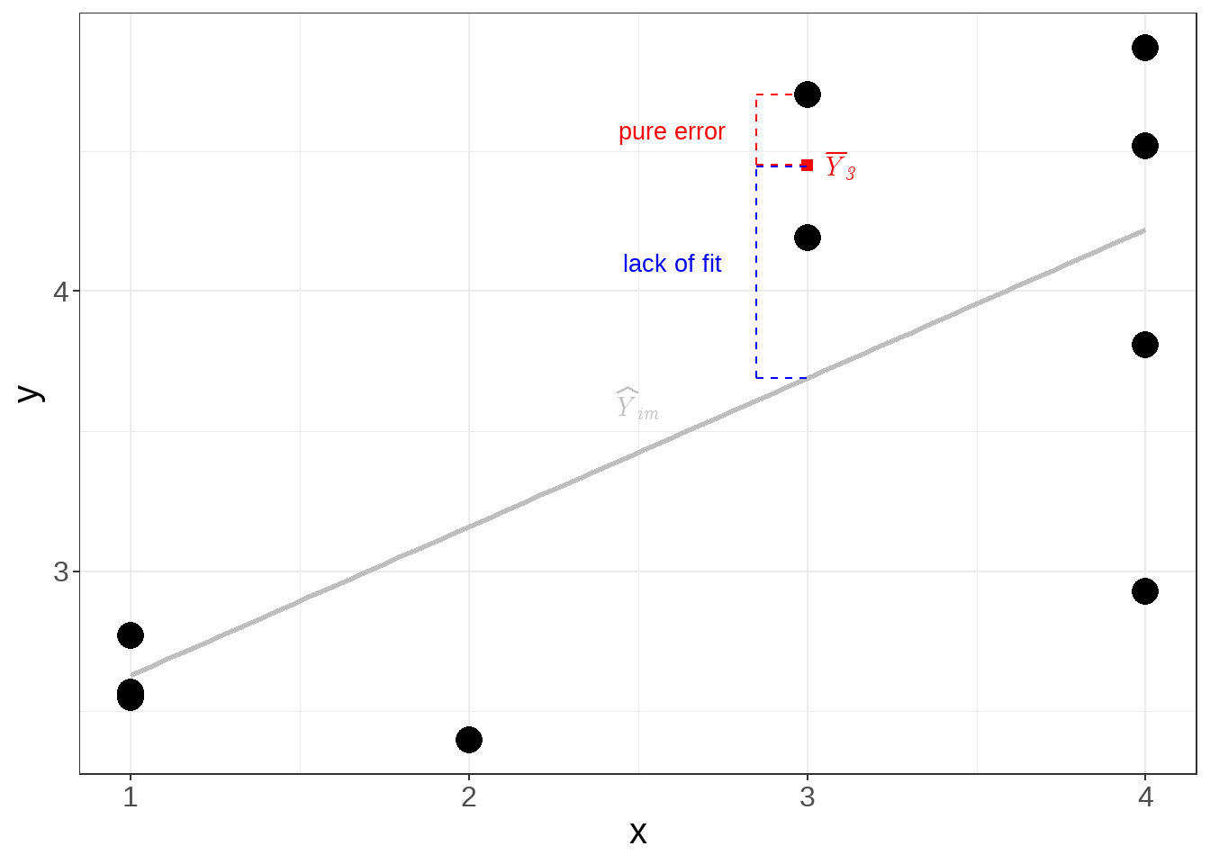
In the Lack of Fit Test, we further decompose the SSE into two components:
\[ SSE = SSPE + SSLF \]
\(SSPE\): Pure Error Sum of Squares, which measures variation among replicates (observations with the same predictor value).
\(SSLF\): Lack-of-Fit Sum of Squares, which measures variation between the fitted regression line and the group means.
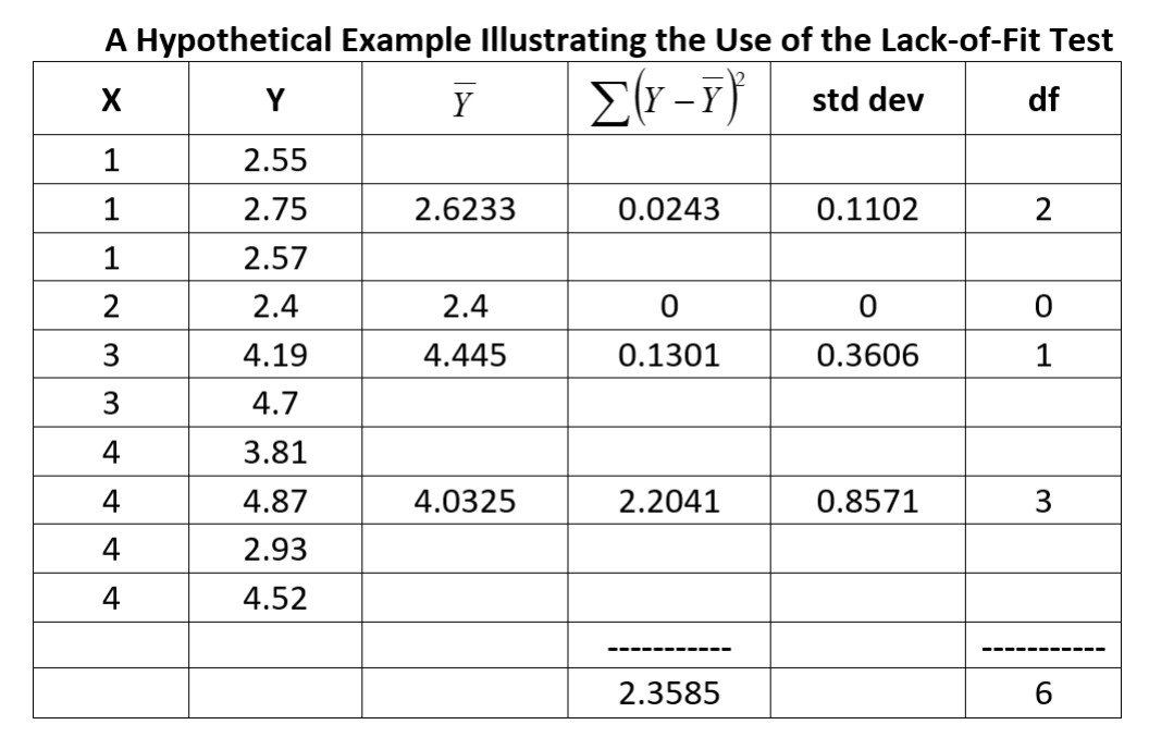
ANOVA table for Testing Lack-of-fit
Let \(Y_{im}\) denote the \(i^{th}\) observation for the \(m^{th}\) level of \(\textbf{x}\) (whether there is replication or none) where \(i = 1, 2, . . . , n_m\) and \(m = 1, 2, . . . , c\), \(n_m\) is the number of replicates for the \(m^{th}\) level of \(\textbf{x}\), and \(c\) is the number of unique predictor levels.
The following is the ANOVA table for testing lack-of-fit for MLRM
| Source of Variation | Sum of Squares | df | Mean Square | F |
|---|---|---|---|---|
| Regression | SSR | p-1 | MSR | \(F_2=\frac{MSR}{MSE}\) |
| Error | SSE | n-p | MSE | |
| Lack of Fit | SSLF | c-p | MSLF | \(F_1=\frac{MSLF}{MSPE}\) |
| Pure Error | SSPE | n-c | MSPE | |
| Total | SST | n-1 |
where
- \(SSE = \sum_{m=1}^c\sum_{i=1}^{n_m}(Y_{im}-\hat{Y}_{im})^2 =SSLF+SSPF\)
- \(SSPE=\sum_{m=1}^c\sum_{i=1}^{n_m}(Y_{im}-\bar{Y}_m)^2\)
- \(SSLF=\sum_{m=1}^c\sum_{i}^{n_m}(\bar{Y_{m}}-\hat{Y}_{im})^2\)
- \(MSLF=\frac{SSLF}{c-p}\)
- \(MSPE=\frac{SSPE}{n-c}\)
Simple Illustration in Simple Linear Regression:
The F-test for Lack-of-Fit
Definition 5.8
The hypotheses for the classic lack-of-fit test are given by
\(Ho\): The relationship assumed in the model is reasonable (i.e. no lack of fit)}
\(Ha\): The relationship assumed in the model is not reasonable (i.e. there is lack of fit)
The test statistic is \(F_1=\frac{SSLF/(c-p)}{SSPE/(n-c)}\sim F_{(c-p,n-c)}\)
We Reject Ho if \(F_1>F_{\alpha, (c-p) , (n-c) }\)
If the test is
significant - this indicates that the model appears to be inadequate. Attempts should be made to discover where and how the inadequacy occurs.
not significant - this indicates that there appears to be no reason to doubt the adequacy of the model and both the pure error and lack-of-fit mean squares can be used as estimators of \(\sigma^2\). The usual practice is to use the \(MSE\) over \(MSPE\) as an estimator of \(\sigma^2\) because the former contains more degrees of freedom.
Remarks:
Not all levels of \(x\) need have repeat observations. Repeat observations at only one or some levels of \(x\) will be adequate.
The F-test for lack-of-fit falls into the framework of a GLT. The full model is: for each level \(x_m\) , \(Y\) is normal with mean \(E(Y_m)\) and variance \(\sigma^2\).
The F-test for significance of the overall regression is valid only if no lack-of-fit is exhibited by the model.
The F-test for lack-of-fit can be used to test the aptness of other regression functions, not just the linear function. This can be useful in Testing for Nonlinearity
The alternative hypothesis includes all regression functions other than a linear one.
Repeat observations are most valuable whenever we are not certain of the nature of the regression function. If at all possible, provision should be made for some replications.
Observations at the same level of \(x\) are genuine repeats only if they involve independent trials with respect to the error term.
Limitations:
The test needs replication in X . This is hard to establish when the values of the X ’s are not predetermined. This is not a problem in experimental designs.
Certain modifications of the test has been proposed for this limitation. Daniel and Woods (1980) has proposed the concept of “near replicates” to establish replications. More solutions has been proposed by Joglekar et. al. (1989).
The test requires that the model follows the normality and homoskedasticity assumption.