Chapter 4 Least Squares Theory
Click for a quick review
Review of the Regression Model
- The regression model: \(\textbf{Y}=\textbf{X}\boldsymbol{\beta}+\boldsymbol{\varepsilon}\), where \(\varepsilon_i\overset{iid}{\sim}N(0,\sigma^2)\)
- We can write the (multivariate) distribution of the error vector as \(\boldsymbol{\varepsilon}\sim N_n(\textbf{0},\sigma^2\textbf{I})\)
- It follows that the distribution of the response vector is \(\textbf{Y}\sim N_n(\textbf{X}\boldsymbol{\beta},\sigma^2\textbf{I})\), since we assume that the independent variables are predetermined or constant.
- Note that the design matrix \(\textbf{X}\) may be written as
\[ \textbf{X} = \begin{bmatrix} \textbf{x}'_1\\ \textbf{x}'_2\\ \vdots\\ \textbf{x}'_n\\ \end{bmatrix}\quad \text{with each element} \quad \textbf{x}'_i=\begin{bmatrix} 1 & X_{i1} & X_{i2} \cdots X_{ik} \end{bmatrix} \]
The Response Variable
\(E(\textbf{Y}) = \textbf{X}\boldsymbol{\beta}\) and \(Var(\textbf{Y}) = \sigma^2\textbf{I}\)
Note that, \(E(Y_i)\) is really \(E (Y_i | \textbf{x}_i )\) which is the mean of the probability distribution of \(Y\) corresponding to the level \(\textbf{x}_i\) of the independent variables. For simplicity’s sake, we will assume \(\textbf{x}_i\) to be constants and denote the said mean simply by \(E(Y_i)\).
The OLS estimator of the coefficient vector
- The least squares estimator of \(\boldsymbol{\beta}\) is given by \(\hat{\boldsymbol{\beta}} = (\textbf{X}'\textbf{X})^{−1}\textbf{X}'\textbf{Y}\)
- The OLS estimator \(\hat{\boldsymbol{\beta}}\) is unbiased for \(\boldsymbol\beta\).
- The variance-covariance matrix of \(\hat{\boldsymbol{\beta}}\) is given by \(\sigma^2(\textbf{X}'\textbf{X})^{-1}\)
4.1 Fitted Values and Residuals
Definition 4.1 (Fitted Values) The fitted values of \(Y_i\) denoted by \(\widehat{E(\textbf{Y})}\) or \(\hat{\textbf{Y}}\) is given by:
\[
\widehat{E(\textbf{Y})} = \hat{\textbf{Y}} = \textbf{X}\hat{\boldsymbol{\beta}} = \textbf{X}(\textbf{X}'\textbf{X})^{−1}\textbf{X}'\textbf{Y}
\]
- Remark: \(\hat{Y_i}\) is the point estimator of the mean response given values of the independent variables \(\textbf{x}_i\)
Definition 4.2 (Hat Matrix) The matrix given by \(\textbf{X}(\textbf{X}'\textbf{X} )^{−1}\textbf{X}'\) is usually referred to as the hat matrix and sometimes denoted by \(\textbf{H}\). Also called the projection matrix denoted by \(\textbf{P}\).
- With this, we can look at the fitted values as \(\hat{\textbf{Y}}=\textbf{HY}\)
- The hat matrix is symmetric and idempotent
Definition 4.3 (Residuals) The residuals of the fitted model, denoted by \(\textbf{e}\), is given by \[\begin{align} \textbf{e} & = \textbf{Y} − \hat{\textbf{Y}}=\textbf{Y} − \textbf{X}\hat{\boldsymbol{\beta}} \\ &=\textbf{Y} − \textbf{X}(\textbf{X}'\textbf{X} )^{−1}\textbf{X}'\textbf{Y} \\ &=(\textbf{I}-\textbf{X}(\textbf{X}'\textbf{X} )^{−1}\textbf{X}')\textbf{Y} \end{align}\]
Remarks:
- Take note that \(\boldsymbol{\varepsilon}= \textbf{Y} − \textbf{X}\boldsymbol{\beta}\), which implies that it is a function of unknown parameters \(\boldsymbol{\beta}\) and is also therefore unobservable.
- On the other hand, residuals are observable.
- We can look at residuals as the ”estimates” of our error terms. (but not really…)
- Note that departures from the assumptions on the error terms will likely reflect on the residuals.
- To validate assumptions on the error terms, we will validate the assumptions on the residuals instead, since the true errors \(\boldsymbol{\varepsilon}\) are not directly observable.
- Using the hat matrix, we can express the residual vector as \(\textbf{e} = (\textbf{I} − \textbf{H})\textbf{Y}\)
Extra reading: What is the difference between the residual and the error term?
One misconception about the residual and the error terms is that they are the same.
Error term is the difference between the actual observed values and the theoretical line: \[\varepsilon_i=Y_i-(\beta_0+\beta X_i)\]
Residual is the difference between the actual observed values and the fitted line: \[e_i=Y_i-(\hat{\beta}_0+\hat{\beta} X_i)\]
Other misconceptions include:
“Residuals are the observed values of the random variable \(\varepsilon\)”.
Note that residual is also a random variable.“The residual is an estimator of the error term.”
It is not. The error term is not a parameter to estimate.The values of the error term cannot be observed. We just use the residual as “proxy” to the error term since this is the random variable where we can get observed values.
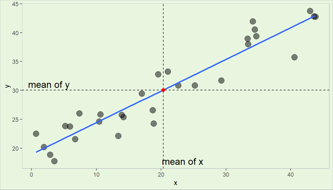
To visualize, let the random variable \(Y_i\) be defined by the equation and random process \[ Y_i=15+2X_i+\varepsilon_i,\quad \quad \varepsilon_i\sim N(0,\sigma=10) \]
x     <- 1:40 # assume that x are predetermined
error <- rnorm(40,0,10) # we can't observe these values naturally in the real world.
y     <- 15 + 2*x + error
We plot the points \(Y_i\) and the theoretical line without the errors \(y=15 + 2x\)
ggplot()+
    geom_point(aes(x=x,y=y)) +        # points (y_i, x_i)
    geom_abline(intercept=15,slope=2) # line of y = 15+2x
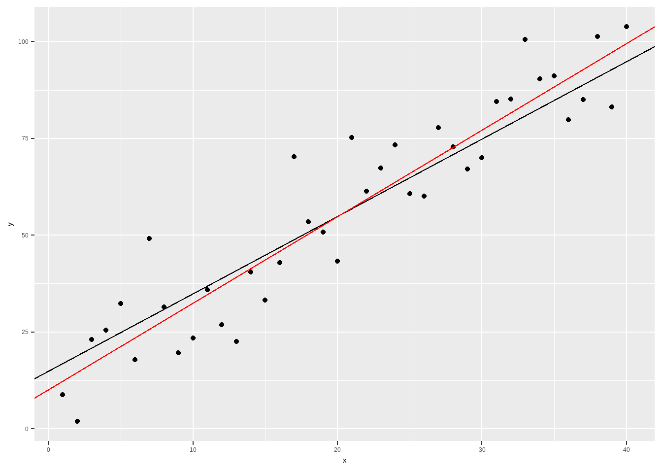
Now, we fit a line that passes through the center of the points using OLS estimation of the regression coefficients.
##
## Call:
## lm(formula = y ~ x)
##
## Coefficients:
## (Intercept)            x
##      10.242        2.236
Now, plotting the fitted line \(\hat{y}=\hat{\beta_0}+\hat{\beta_1}x\)
ggplot() +

    # points (y_i, x_i)
    geom_point(aes(x=x,y=y)) +

    # line of y = 15+2x
    geom_abline(intercept=15,slope=2) +

    # fitted line
    geom_abline(intercept=coef(mod)[1], slope=coef(mod)[2], color = "red")
The error \(\varepsilon_i\) is the (vertical) distance between the black line and the point \(y_i\).
The residual \(e_i\) is the (vertical) distance between the red line and the point \(y_i\). The values will also depend on the line estimation procedure that will be used.
The following table summarizes the dataset used, the errors, and the residuals.
y x error residual 8.739827 1 -8.2601734 -3.7376207 1.901259 2 -17.0987407 -12.8119309 23.108018 3 2.1080182 6.1590850 25.458703 4 2.4587029 6.2740266 32.310937 5 7.3109367 10.8905175 17.798514 6 -9.2014856 -5.8576479 49.078102 7 20.0781016 23.1861964 31.393114 8 0.3931142 3.2654660 19.564041 9 -13.4359588 -10.7993500 23.420723 10 -11.5792768 -9.1784110 35.915405 11 -1.0845947 1.0805281 26.867971 12 -12.1320294 -10.2026496 22.539348 13 -18.4606525 -16.7670157 40.439170 14 -2.5608296 -1.1029358 33.212216 15 -11.7877840 -10.5656332 42.906307 16 -4.0936926 -3.1072847 70.219442 17 21.2194416 21.9701065 53.433670 18 2.4336705 2.9485923 50.819296 19 -2.1807042 -1.9015253 43.330222 20 -11.6697782 -11.6263423 75.258913 21 18.2589129 18.0666058 61.299762 22 2.2997625 1.8717124 67.353457 23 6.3534570 5.6896639 73.305379 24 10.3053786 9.4058425 60.684641 25 -4.3153594 -5.4506385 60.143128 26 -6.8568717 -8.2278938 77.714033 27 8.7140333 7.1072682 72.787178 28 1.7871783 -0.0553298 67.080356 29 -5.9196442 -7.9978953 70.021683 30 -4.9783165 -7.2923106 84.489306 31 7.4893065 4.9395695 85.185146 32 6.1851464 3.3996663 100.580921 33 19.5809210 16.5596980 90.413510 34 7.4135102 4.1565442 91.159419 35 6.1594190 2.6667100 79.755801 36 -7.2441991 -10.9726511 85.025867 37 -3.9741327 -7.9383277 101.283455 38 10.2834547 6.0835167 83.147365 39 -9.8526351 -14.2883161 103.831818 40 8.8318182 4.1603942
The following relative frequency histograms of the error and the residuals show that they almost follow the same shape.
The closer the fitted line to the theoretical line is, the more likely that the two histograms will look identical

Exercise 4.1 Show that the hat matrix is symmetric and idempotent.
Exercise 4.2 Show that the rank of \(\textbf{I}-\textbf{H}\) is \(n-p\).
Theorems
The following theorems will be important for later results. Try to prove them all as your practice.
Theorem 4.1 \[ \hat{\boldsymbol{\beta}}=\boldsymbol{\beta}+(\textbf{X}'\textbf{X})^{-1}\textbf{X}'\boldsymbol{\varepsilon} \] That is, the OLS estimator can be thought of as a linear function of the error terms and the model parameters.
Theorem 4.2 The sum of the observed values \(Y_i\) is equal to the sum of the fitted values \(\hat{Y_i}\)
\[
\sum_{i=1}^nY_i=\sum_{i=1}^n\hat{Y_i}
\]
Hint for Proof
Use the first normal equation in OLS
Theorem 4.3 The expected value of the vector of residuals is a null vector. That is, \[ E(\textbf{e})=\textbf{0} \]
Theorem 4.4 The sum of the squared residual is a minimum. That is, \(\textbf{e}'\textbf{e}\) is the minimum value of \(\boldsymbol\varepsilon'\boldsymbol\varepsilon\)
Theorem 4.5 The sum of the residuals in any regression model that with an intercept \(\beta_0\) is always equal to 0. \[ \sum_{i=1}^n e_i = \textbf{1}'\textbf{e} = \textbf{e}'\textbf{1}=0 \]
Hint for Proof
Use the Theorem 4.2
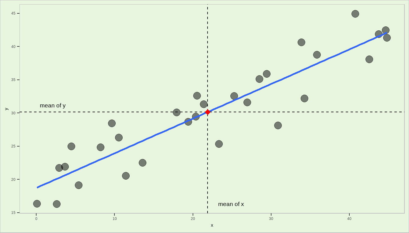
Theorem 4.6 The least squares regression line always passes through the centroid (the point comprising of the means of the dependent and independent variables). That is, if \((\bar{y},\bar{x_1},\bar{x_2},\cdots,\bar{x_k})\) is the centroid of the the dataset, the following equation is true: \[ \bar{y}=\hat{\beta}_0 + \hat{\beta}_1 \bar{x}_1 + \hat{\beta}_2 \bar{x}_2 +\cdots + \hat{\beta}_k \bar{x}_k \]
Visualization
Theorem 4.7 The sum of the residuals weighted by the corresponding value of the regressor variable is always equal to zero. That is,
\[
\sum_{i=1}^nX_{ij}e_{i}=0 \quad \text{or}
\quad \textbf{X}'\textbf{e}=\textbf{0}
\]
Hint for Proof
Use result from Theorem 4.5, then use the 2nd to (k+1)th normal equations. For every variable \(X_{ij}\), use equation \(j+1\).
Theorem 4.8 The sum of the residuals weighted by the corresponding value of the fitted value is always equal to 0. That is, \[ \sum_{i=1}^n\hat{Y_i}e_i=\textbf{e}'\hat{\textbf{Y}}=0 \]
Hint for Proof
Use previous theorem on sum of residual \(e_j\) and sum of residual \(e_i\) weighted by \(X_{ij}\)
Theorem 4.9
The residual and independent variables are uncorrelated. That is, assuming that \(Xs\) are random again, \[ \rho(X_{ij},e_{ij})=0 \]
Theorem 4.10 The residual and the fitted values are uncorrelated.
\[ \rho(\hat{Y_i},e_i)=0 \]
Remarks:
- One reason why the \(X\)s are required to be uncorrelated (or linearly independent to each other) is to ensure proper conditioning of \(\textbf{X}'\textbf{X}\) and hence, stability of the inverse that will imply stability of the parameter estimates.
- Note that aside from estimating \(\boldsymbol{\beta}\), we also need to estimate \(\sigma^2\) to make inferences regarding the model parameters.
- Before we estimate \(\sigma^2\), we need to discuss first the the sum of squares of the regression analysis.
Exercise 4.3 Assume that the design matrix \(\textbf{X}\) is only a vector of 1s. That is, there is no independent variable, and you will only estimate the intercept \(\beta_0\).
Show that \(\hat{Y}_i = \bar{Y} = \hat{\beta}_0\quad \forall\quad i\).
Exercise 4.4 Under the normal error assumption of the linear regression, derive the distribution of the coefficient estimator vector \(\hat{\boldsymbol{\beta}}\).
.
4.2 Sum of Squares and Mean Squares
After fitting a regression model, we want to know: How much of the variation in \(Y\) is explained by the model, and how much is left as error?
We measure this using sum of squares, which splits the total variation in \(Y\) into two parts:
Regression sum of squares \((SSR)\): variation explained by the predictors,
Error sum of squares \((SSE)\): unexplained variation.
Dividing these by their degrees of freedom gives the mean squares, which are used to estimate the error variance \(\sigma^2\) and to test whether the regression model explains a significant portion of the variation, which will be discussed in the next chapter Analysis of Variance.
Sum of Squares
We start with the observed deviations of \(Y_i\) around the observed mean: \(Y_i-\bar{Y}\).
Definition 4.4 (Total Sum of Squares) The measure of total variation is denoted by \[ SST =\sum_{i=1}^n (Y_i-\bar{Y})^2 \]
- \(SST\) is the total corrected sum of squares
- If all \(Y_i\)s are the same, then \(SST=0\)
- The greater the variation of \(Y_i\)s, the greater \(SST\)
- In analysis of variance, we want to find the source of this variation
Now, recall that \(\hat{Y_i}\)s are the fitted values. Other than the variation of the observed \(Y_i\)s, we can also measure the variation of the \(\hat{Y_i}\)s. Note that the mean of the fitted values is also \(\bar{Y}\). We can now explore the deviation \(\hat{Y_i}-\bar{Y}\)
Definition 4.5 (Regression Sum of Squares) The measure of variation of the fitted values due to regression is denoted by
\[ SSR = \sum_{i=1}^n (\hat{Y_i}-\bar{Y})^2 \]
\(SSR\) is the sum of squares due to regression
This measures the variability of \(Y\) associated with the regression line or due to changes in the independent variables.
Sometimes referred to as “explained sum of squares”
If the \(X\)s explain the variation of \(Y\) (i.e. the model is good), then we expect that this measure is to be large.
Finally, recall that the quantity \(Y_i-\hat{Y_i}\) is the residual, or the difference between the observed values and the predicted values when the independent variables are taken into account.
Definition 4.6 (Sum of Squared Deviations) The measure of variation of the \(Y_i\)s that is still present when the predictor variable \(X\) is taken into account is the sum of the squared deviations
\[ SSE=\sum_{i=1}^n(Y_i-\hat{Y_i})^2 \]
- \(SSE\) is the sum of squares due to error
- Mathematically, the formula is the sum of squares of the residuals \(e_i\), not the error. That is why some software outputs show “Sum of Squares from Residuals”.
- It still measures the variability of \(Y\) due to causes other than the set of independent variables.
- Sometimes referred to as ”unexplained sum of squares”
- If the independent variables predict the response variable well, then this quantity is expected to be small.
Theorem 4.11 (Decomposition of Sum of Squares in Least Squares Regression) Under the least squares theory, the sum of squares can be partitioned as
\[\begin{matrix} \sum_{i=1}^n(Y_i-\bar{Y})^2&=& \sum_{i=1}^n(\hat{Y_i}-\bar{Y_i})^2&+& \sum_{i=1}^n(Y_i-\hat{Y_i})^2\\ SST &=& SSR &+& SSE \end{matrix}\]Proof
First express \(Y_i-\bar{Y}\) as a sum of two differences by adding and subtracting \(\hat{Y_i}\), then square both sides.
\[\begin{align} (Y_i-\bar{Y})^2 &= [(Y_i-\bar{Y})+(\hat{Y_i}-\hat{Y_i})]^2\\ &= [(Y_i-\hat{Y_i}) + (\hat{Y_i}-\bar{Y})]^2\\ &= (Y_i-\hat{Y_i})^2+(\hat{Y_i}-\bar{Y})^2 + 2(Y_i-\hat{Y_i})(\hat{Y_i}-\bar{Y})\\ &= (Y_i-\hat{Y_i})^2+(\hat{Y_i}-\bar{Y})^2 + 2(Y_i-\hat{Y_i})\hat{Y_i} - 2(Y_i-\hat{Y_i})\bar{Y}\\ &= (Y_i-\hat{Y_i})^2+(\hat{Y_i}-\bar{Y})^2 + 2 e_i \hat{Y_i} - 2 e_i \bar{Y} \end{align}\]
Now getting summation of both sides.
\[\begin{align} \sum_{i=1}^n(Y_i-\bar{Y})^2 &=\sum_{i=1}^n(Y_i-\hat{Y_i})^2 + \sum_{i=1}^n(\hat{Y_i}-\bar{Y})^2 +2\sum_{i=1}^n e_i \hat{Y_i}+2\bar{Y}\sum_{i=1}^n e_i \\ &=\sum_{i=1}^n(Y_i-\hat{Y_i})^2 + \sum_{i=1}^n(\hat{Y_i}-\bar{Y})^2\end{align}\]
Since \(\sum_{i=1}^n\hat{Y}_ie_i=0\) and \(\sum_{i=1}^ne_i=0\) from Theorems 4.8 and 4.5 respectively.
\(\blacksquare\)
Matrix form of the sums of squares
- \(SST=(\textbf{Y}-\bar{Y}\textbf{1})'(\textbf{Y}-\bar{Y}\textbf{1})\)
- \(SSR = (\hat{\textbf{Y}}-\bar{Y}\textbf{1})'(\hat{\textbf{Y}}-\bar{Y}\textbf{1})\)
- \(SSE = (\textbf{Y}-\hat{\textbf{Y}})'(\textbf{Y}-\hat{\textbf{Y}})\)
Exercise 4.5 Show the following (quadratic form of the sum of squares):
- \(SST = \textbf{Y}'(\textbf{I}-\bar{\textbf{J}})\textbf{Y}\)
- \(SSR = \textbf{Y}'(\textbf{H}-\bar{\textbf{J}})\textbf{Y}\)
- \(SSE = \textbf{Y}'(\textbf{I}-\textbf{H})\textbf{Y}\)
Breakdown of Degrees of Freedom
Let \(p=k+1\), the number of coefficients to be estimated (\(\beta_0,\beta_1,...,\beta_k\)) , or the number of columns in the design matrix.
- \(SST=\sum_{i=1}^n(Y_i-\bar{Y})^2\)
- \(n\) observations but \(1\) linear constraint due to the calculation and inclusion of the mean
- \(n-1\) degrees of freedom
- \(SSR=\sum_{i=1}^n(\hat{Y_i}-\bar{Y})^2\)
- \(p\) degrees of freedom in the regression parameters, one is lost due to linear constraint
- \(p-1\) degrees of freedom
- \(SSE=\sum_{i=1}^n(Y_i-\hat{Y_i})^2\)
- \(n\) independent observations but \(p\) linear constraints arising from the estimation of \(\beta_0,\beta_1,...,\beta_k\)
- \(n-p\) degrees of freedom
In classical linear regression, the degrees of freedom associated with a quadratic form involving \(\textbf{Y}\) is equal to the rank of the matrix involved in the quadratic form.
This will be explained more in Stat 147.
Mean Squares
In regression, sums of squares measure how much variation is explained or left unexplained by a model.
However, sums of squares by themselves cannot be compared directly because they depend on sample size and the number of model parameters.
To make meaningful comparisons, we convert each sum of squares into an average amount of variation per degree of freedom. These quantities are called the mean squares.
Definition 4.7 (Mean Squares) The mean squares in regression are the sum of squares divided by their corresponding degrees of freedom.
\[ MST = \frac{SST}{n-1}\quad MSR = \frac{SSR}{p-1} \quad MSE = \frac{SSE}{n-p} \]
The ratio of these \(MSR\) and \(MSE\) follows a distribution, which you will be asked to prove in Exercise 4.6 later (under \(Ho\)). This will be useful in assessing if our model is sufficient in explaining variation in \(Y\).
Estimation of \(Var(\varepsilon)\) and \(Var(\hat{\boldsymbol{\beta}})\)
Now that we already finished the discussion on mean squares, we now have a way to estimate the error term variance \(\sigma^2\). One possible estimator is the \(MSE\).
Theorem 4.12 \(MSE\) is an unbiased estimator of \(\sigma^2\)
More properties regarding \(MSE\) as an estimator of \(\sigma^2\) will be discussed later in Section 4.4.
Furthermore, from this, we can also estimate the variance and standard error of the OLS estimators.
Recall that \(Var(\hat{\boldsymbol\beta})=\sigma^2(\textbf{X}'\textbf{X})^{−1}\) from Theorem 3.3.
By Theorem 4.12, \(MSE\) is a possible estimator of \(\sigma^2\), which gives us a possible estimator of the variance-covariance matrix \(Var(\hat{\boldsymbol\beta})\).
Definition 4.8 an estimator of \(Var(\hat{\boldsymbol\beta})\) is given by
\[ \widehat{Var(\hat{\boldsymbol{\beta}})} = \widehat{\sigma^2}(\textbf{X}'\textbf{X})^{−1}=MSE (\textbf{X}'\textbf{X})^{−1} \]
And for the standard error of each individual \(\hat{\beta}_j\), we have the following:
Definition 4.9 an estimator for the standard deviation of \(\hat{\beta_j}\) is the square root of the \((j+1)^{th}\) diagonal element of \(\widehat{Var}({\hat{\boldsymbol{\beta}}})\). In matrix form:
\[ \widehat{s.e\left(\hat{\beta}_j\right)}=\sqrt{\underline{e}_{j+1}'\widehat{Var}({\hat{\boldsymbol{\beta}}})\underline{e}_{j+1}}=\sqrt{MSE\underline{e}_{j+1}'(\textbf{X}'\textbf{X})^{−1}\underline{e}_{j+1}} \]
where \(\underline{e}_k\) is a vector of \(0\)s with \(1\) on the \(k^{th}\) element.
This will be useful later Inference about the Slope Parameters.
Sampling Distribution of the Sum of Squares while Assuming Same Means of \(Y_i|\textbf{x}\)
It will also be useful to define the sampling distribution of the statistics that can be obtained from the sum of squares.
Theorem 4.13 (Cochran's Theorem) If all \(n\) observations \(Y_i\) come from the same normal distribution with same mean \(\mu\) and variance \(\sigma^2\) and \(SST\) is decomposed into k sums of squares \(SS_j\) , each with \(\text{df}_j\) , then the \(\frac{SS_j}{\sigma^2}\) terms are independent \(\chi^2\) random variables with \(\text{df}_j\) if \(\sum_{j=1}^k\text{df}_j\text{s} = \text{df}\text{ of } SST = n-1\).
If all observations comes from the same normal distribution with SAME PARAMETERS regardless of \(i\), that is \(Y_i \overset{iid}{\sim} N(\beta_0,\sigma^2)\), then
\[ \frac{SST}{\sigma^2} \sim \chi^2_{(n-1)} \quad \frac{SSR}{\sigma^2} \sim \chi^2_{(p-1)} \quad \frac{SSE}{\sigma^2} \sim \chi^2_{(n-p)} \]
Exercise 4.6 Assuming normality of errors and \(\beta_1=\beta_2=\cdots=\beta_k=0\), show that \(MSR/MSE\) follows the \(F\) distribution.
This will be useful later in Analysis of Variance.
4.3 Coefficient of Multiple Determination
Definition 4.10 (Coefficient of Multiple Determination) The coefficient of multiple determination of \(Y\) associated with the use of the set of independent variables \((X_1, X_2, . . . , X_k )\) denoted by \(R^2\) or \(R^2_{Y.1,2,...,k}\) is defined as \[ R^2=R^2_{Y.1,2,...,k}=\frac{SSR(X_1,X_2,...,X_k)}{SST}=1-\frac{SSE(X_1,X_2,...,X_k)}{SST} \]
Remarks:
The coefficient of multiple determination measures the percentage of variation in Y than can be explained by the \(X\)s through the model.
For \(R^2\), the larger the better. However, high value of \(R^2\) does not imply usefulness of the model.
\(R^2\) increases as more variables are included in the model (cross-classified data)
\(0 \leq R^2 \leq 1\)
\(R^2 = r^2\) when \(k = 1\), where \(r\) is the Pearson’s r
If the intercept is dropped from the model, \(R^2 = SSR/SST\) is an incorrect measure of coefficient of determination.
Exercise 4.7
Read: What is overfitting?
In statistical modelling, there is this problem called “overfitting”. This occurs if the model becomes more deterministic that it may not describe the statistical relationship of the dependent and independent variables.
Common indication for this is too high \(R^2\) (close to 1).
This further implies that the model is good for the collected data, but may not perform well for new data. A good statistical model must have enough elbow room for possible errors in data.
In the following exercise, we show that overfitting exists for a specific case based on the number of observed values in the collected dataset.
Suppose that the observed values for your dependent variable are not constant and the observed values of the independent variables are linearly independent.
Show that if the number of observations and number of parameters to be estimated are equal to each other (\(n=p\)), then \(R^2=1\)
Recall that as more variables are included in the model, it is expected that the \(R^2\) increases. We do not want this, since we want to penalize adding variables that do not explain the dependent variable well. The following definition is a more conservative measure of coefficient of determination.
Definition 4.11 (Adjusted Coefficient of Determination) The adjusted coefficient of determination denoted by \(R_a^2\) is defined as
\[ R^2_a=1-\frac{MSE}{MST}=1-\frac{SSE/(n-p)}{SST/(n-1)} \]
Example in R
In R, both the Multiple R-squared and Adjusted R-squared are shown using the summary() function. In this example, note that mod_anscombe is an lm object from the ANOVA example.
##
## Call:
## lm(formula = income ~ education + young + urban, data = Anscombe)
##
## Residuals:
##     Min      1Q  Median      3Q     Max
## -438.54 -145.21  -41.65  119.20  739.69
##
## Coefficients:
##              Estimate Std. Error t value Pr(>|t|)
## (Intercept) 3011.4633   609.4769   4.941 1.03e-05 ***
## education      7.6313     0.8798   8.674 2.56e-11 ***
## young         -6.8544     1.6617  -4.125  0.00015 ***
## urban          1.7692     0.2591   6.828 1.49e-08 ***
## ---
## Signif. codes:  0 '***' 0.001 '**' 0.01 '*' 0.05 '.' 0.1 ' ' 1
##
## Residual standard error: 259.7 on 47 degrees of freedom
## Multiple R-squared:  0.7979, Adjusted R-squared:  0.785
## F-statistic: 61.86 on 3 and 47 DF,  p-value: 2.384e-16
Using the Adjusted \(R^2\), 78.5% of the variation in income can be explained by the model.
4.4 Properties of the Estimators of the Regression Parameters
In the following section, we will show that the OLS estimator \(\hat{\boldsymbol{\beta}}\) is also the BLUE, MLE, and UMVUE of \(\boldsymbol{\beta}\). Estimators for the variance \(\sigma^2\) are presented as well.
Best Linear Unbiased Estimator of \(\boldsymbol{\beta}\)
Theorem 4.14 (Gauss-Markov Theorem)
Under the classical conditions of the multiple linear regression model (i.e., \(E(\boldsymbol{\varepsilon}) = \textbf{0}\), \(Var(\boldsymbol{\varepsilon}) = \sigma^2\textbf{I}\), not necessarily normal), the least squares estimator \(\hat{\boldsymbol\beta}\) is the best linear unbiased estimator (BLUE) of \(\boldsymbol{\beta}\). This means that among all linear unbiased estimators of \(\beta_j\), \(\hat{\beta_j}\) has the smallest variance, \(j = 0, 1, 2, ..., k\).
Hint and Definitions
An estimator \(\tilde{\boldsymbol\beta}\) is linear if it is a linear function of the observed data \(\textbf{Y}\): \(\tilde{\boldsymbol\beta}=\textbf{A}\textbf{Y}\)
\(\tilde{\boldsymbol\beta}\) is unbiased if: \(E(\tilde{\boldsymbol\beta})=\boldsymbol{\beta}\)
For a linear estimator \(\tilde{\boldsymbol\beta}=\textbf{A}\textbf{Y}\), we have: \(E(\tilde{\boldsymbol\beta})=\textbf{A}E(\textbf{Y}) =\textbf{AX}\boldsymbol{\beta}\)
For \(\tilde{\boldsymbol\beta}\) to be unbiased, some case must be assumed.
Among all linear unbiased estimators, the best one has the minimum variance. That is, the difference of the diagonal elements \(Var(\overset{\sim}{\boldsymbol\beta})\) and \(Var(\hat{\boldsymbol\beta})\) must all be greater than or equal to 0. In the matrix sense: \(Var(\tilde{\boldsymbol\beta})-Var(\hat{\boldsymbol\beta}) \text{ is positive definite}\)
To summarize, we want to show:
For any linear unbiased estimator \(\tilde{\boldsymbol\beta}=\textbf{A}\textbf{Y}\), the difference in variance matrices
\[ Var(\tilde{\boldsymbol\beta}) - Var(\hat{\boldsymbol{\beta}}) \] is positive-definite (i.e. all diagonal entries \(\geq0\))
Full Proof
Step 1: Show that OLS is linear and unbiased estimator
\[ \hat{\boldsymbol{\beta}}=\underbrace{(\textbf{X}'\textbf{X})^{-1}\textbf{X}'}\textbf{Y} \] This is linear in \(\textbf{Y}\)
Checking for unbiasedness: \[ \begin{align} E(\hat{\boldsymbol{\beta}})=&(\textbf{X}'\textbf{X})^{-1}\textbf{X}'E(\textbf{Y})\\ =&\underset{\textbf{I}}{\underbrace{(\textbf{X}'\textbf{X})^{-1}\textbf{X}'\textbf{X}}}\boldsymbol{\beta}\\ =&\boldsymbol{\beta} \end{align} \] So, \(\hat{\boldsymbol{\beta}}\) is linear and unbiased.
Step 2: Consider any other linear unbiased estimator
Let \(\tilde{\boldsymbol{\beta}}=\textbf{AY}\) be another linear estimator.
Then, \(E(\tilde{\boldsymbol{\beta}})=\textbf{A}E(\textbf{Y})=\textbf{AX}\boldsymbol{\beta}\).
Which gives us the unbiasedness condition \(\textbf{AX}=\textbf{I}_p\) since the relationship \(\textbf{AX} \boldsymbol{\beta}=\boldsymbol{\beta}\) must hold for any possible value of \(\boldsymbol{\beta}\).
Step 3: Variances of the linear unbiased estimators
Let \(\textbf{D}=\textbf{A}-(\textbf{X}'\textbf{X})^{-1}\textbf{X}'\).
Now,
\[\begin{align} \textbf{AA}' &=(\textbf{D}+(\textbf{X}'\textbf{X})^{-1}\textbf{X}')(\textbf{D}+(\textbf{X}'\textbf{X})^{-1}\textbf{X}')'\\ &=(\textbf{D}+(\textbf{X}'\textbf{X})^{-1}\textbf{X}')(\textbf{D}'+\textbf{X}(\textbf{X}'\textbf{X})^{-1})\\ &=\textbf{DD}'+\textbf{D}\textbf{X}(\textbf{X}'\textbf{X})^{-1}+(\textbf{X}'\textbf{X})^{-1}\textbf{X}'\textbf{D}'+(\textbf{X}'\textbf{X})^{-1}\textbf{X}'\textbf{X}(\textbf{X}'\textbf{X})^{-1}\\ &=\textbf{DD}'+\textbf{D}\textbf{X}(\textbf{X}'\textbf{X})^{-1}+(\textbf{X}'\textbf{X})^{-1}\textbf{X}'\textbf{D}'+(\textbf{X}'\textbf{X})^{-1} \end{align}\]
Aside: Recall the unbiasedness condition \(\textbf{AX}=\textbf{I}_p\).
This implies \((\textbf{D}+(\textbf{X}'\textbf{X})^{-1}\textbf{X}')\textbf{X}=\textbf{I}_p\rightarrow\textbf{DX}+\textbf{I}_p=\textbf{I}_p\rightarrow \textbf{DX}=\textbf{0}\)
Going back, we are now left with:
\[ \textbf{AA}' =\textbf{DD}'+(\textbf{X}'\textbf{X})^{-1} \]
Computing for the variance of \(\tilde{\boldsymbol{\beta}}\), we get:
\[\begin{align} Var(\tilde{\boldsymbol{\beta}}) &= \sigma^2\textbf{AA}'\\ &= \sigma^2\textbf{DD}' + \sigma^2(\textbf{X}'\textbf{X})^{-1}\\ &=\sigma^2\textbf{DD}'+Var(\hat{\boldsymbol{\beta}})\\ \end{align}\]
Which now implies \(Var(\tilde{\boldsymbol{\beta}})-Var(\hat{\boldsymbol{\beta}}) = \sigma^2\textbf{DD}'\).
Step 4: a psd matrix
To show that the variances of \(\tilde{\beta}_j\) are larger than \(\hat{\beta}_j\), we just need to show that the diagonals of \(Var(\tilde{\boldsymbol{\beta}})-Var(\hat{\boldsymbol{\beta}})\) are \(\geq 0\), or \(\sigma^2\textbf{DD}'\) is a positive semi-definite matrix.
\(\textbf{DD}'\) is psd if \(\textbf{u}'\textbf{DD}'\textbf{u}\geq0 \quad \forall \textbf{u}\)
Let \(\textbf{v}=\textbf{D}'\textbf{u}\).
\[ \textbf{u}'\textbf{DD}'\textbf{u}=\textbf{v}'\textbf{v} \geq0 \]
Since the inner product \(\textbf{v}'\textbf{v}\) is a sum of squares.
Therefore, \(\textbf{DD}'\) is a positive definite matrix, and also \(\sigma^2\textbf{DD}'\) is psd.
We have shown that the diagonal elements of the variance-matrix of any linear unbiased estimator \(\tilde{\boldsymbol{\beta}}\) are all greater than or equal to the diagonal elements of the variance-covariance matrix of the OLS estimator \(\hat{\boldsymbol{\beta}}\) by showing that \(\sigma^2\textbf{DD}'\) is psd.
Therefore, \(\hat{\boldsymbol{\beta}}\) is the best linear unbiased estimator for \(\boldsymbol{\beta}\) \(\blacksquare\)
Remarks:
- The Gauss-Markov Theorem states that even though the error terms are not normally distributed, the OLS estimator is still a viable estimator for linear regression.
- The OLS estimator will give the smallest possible variance among all linear unbiased estimators of \(\boldsymbol\beta\)
- Any linear combination \(\boldsymbol{\lambda}'\boldsymbol\beta\) of the elements of \(\boldsymbol\beta\), the BLUE is \(\boldsymbol{\lambda}'\hat{\boldsymbol\beta}\)
Maximum Likelihood Estimator of \(\boldsymbol{\beta}\) and \(\sigma^2\)
Theorem 4.15 (MLE of the Regression Coefficients and the Variance)
With assumptions of normality of the error terms, the maximum likelihood estimators (MLE) for \(\boldsymbol{\beta}\) and \(\sigma^2\) are \[
\hat{\boldsymbol{\beta}}=(\textbf{X}'\textbf{X})^{-1}(\textbf{X}'\textbf{Y})
\quad \quad \quad
\widehat{\sigma^2}=\frac{1}{n}\textbf{e}'\textbf{e}=\frac{SSE}{n}=\left(\frac{n-p}{n} \right)MSE
\]
Hint for Proof
Recall: \(Y_i \sim Normal(\textbf{x}_i'\boldsymbol{\beta},\sigma^2)\)
Note: the likelihood function is just the joint pdf, but a function of the parameters, given the values of the random variables.
Since \(Y_i\)s are independent, the joint pdf of \(Y_i\)s is the product
\[ \prod_{i=1}^n f_{Y_i}(y_i)=\prod_{i=1}^n \frac{1}{\sqrt{2\pi\sigma^2}}\exp\left\{-\frac{(y_i-\textbf{x}'_i\boldsymbol{\beta})^2}{2\sigma^2}\right\} \]
Hence, you can show that the likelihood function is given by \[ L(\boldsymbol{\beta},\sigma^2|\textbf{Y},\textbf{X})=(2\pi \sigma^2)^{-\frac{n}{2}}\exp\left\{ -\frac{1}{2\sigma^2}(\textbf{Y}-\textbf{X}\boldsymbol{\beta})'(\textbf{Y}-\textbf{X}\boldsymbol{\beta})\right\} \] Obtain the log-likelihood function (for easier maximization).
The maximum likelihood estimator for \(\boldsymbol{\beta}\) and \(\sigma^2\) are the solutions to the following equations: \[ \frac{\partial\ln(L)}{\partial \boldsymbol{\beta}}=\textbf{0} \quad \frac{\partial\ln(L)}{\partial \sigma^2}=0 \quad \]
Full Proof
Remarks:
- We interpret these as the “most likely values” of \(\boldsymbol{\beta}\) and \(\sigma^2\) given our sample (hence the name maximum likelihood).
- The form implies that the MLE estimator for \(\boldsymbol\beta\) is also the OLS \(\hat{\boldsymbol\beta}\) that we showed in Theorem 3.1.
- Recall that MSE is unbiased for \(\sigma^2\) from Theorem 4.12 and obviously, MSE is not the MLE for \(\sigma^2\). Therefore, the MLE estimator of \(\sigma^2\) is not unbiased with respect to \(\sigma^2\).
- The MLE is rarely used in practice; MSE is the conventional estimator for \(\sigma^2\).
UMVUE of \(\boldsymbol{\beta}\) and \(\sigma^2\) under Normality
Theorem 4.16 (UMVUE of the Regression Coefficients and Variance)
Under the assumption of normal error terms, \((\hat{\beta},MSE)\) is the uniformly minimum variance unbiased estimator (UMVUE) of \((\boldsymbol{\beta} ,\sigma^2)\)
Hint for Proof
We have established that \(\hat{\boldsymbol{\beta}}\) and \(MSE\) are unbiased estimators for \(\boldsymbol{\beta}\) and \(\sigma^2\) respectively.
Thus, we can just use the Lehmann-Scheffé Theorem to determine a joint complete sufficient statistic for \((\boldsymbol{\beta},\sigma^2)\).
If the unbiased estimator \((\hat{\boldsymbol{\beta}}, MSE)\) is a function of the joint CSS, then that estimator is UMVUE for \((\boldsymbol{\beta},\sigma^2)\)
Full Proof
- This implies that among all other unbiased estimator of \((\boldsymbol\beta, \sigma^2)\), \((\hat{\boldsymbol\beta}, MSE)\) will give the smallest variability (and hence, the “most precise” or “reliable”).
- The OLS estimator is also the UMVUE for \(\boldsymbol{\beta}\).
| Parameter | OLS | BLUE | MLE | UMVUE |
|---|---|---|---|---|
| \(\boldsymbol\beta\) | \(\hat{\boldsymbol\beta}\) | \(\hat{\boldsymbol\beta}\) | \(\hat{\boldsymbol\beta}\) | \(\hat{\boldsymbol\beta}\) |
| \(\sigma^2\) | - | - | \(\widehat{\sigma^2}=\left(\frac{n-p}{n}\right)MSE\) | \(MSE\) |
Exercise 4.9
Show that the MLE of \(\sigma^2\) is asymptotically unbiased as \(n\rightarrow \infty\).
Show that the variance of the MLE of \(\sigma^2\) approaches 0 as \(n\rightarrow \infty\)
Is the MLE of \(\sigma^2\) MSE-consistent in estimating \(\sigma^2\)? Justify.
4.5 Optional: Standardized Coefficients
Raw (unstandardized) coefficients are unit-dependent. For example, in a fitted model predicting income:
\[ \hat{y}=\hat{\beta}_0 +\hat{\beta}_1(\text{years of education}) + \hat{\beta}_2(\text{age}) \]
\(\hat{\beta}_1\) and \(\hat{\beta}_2\) cannot be compared directly if years of education is in years and age is in decades. Standardizing involves transformation of variables into a common scale (mean 0, standard deviation 1) to make coefficients comparable.
Example in R
The variable wt in the mtcars dataset represents the weight of cars in 1000 lbs. The following is the results of a simple linear regression. Take note of the value of \(\hat{\beta}\)
##
## Call:
## lm(formula = mpg ~ wt, data = mtcars)
##
## Coefficients:
## (Intercept)           wt
##      37.285       -5.344
Now, let’s have another wt variable, but changing the unit to \(lbs\) instead of \(1000 \text{lbs}\)
Now regressing the same variable but in different units:
##
## Call:
## lm(formula = mpg ~ wt_lbs, data = mtcars)
##
## Coefficients:
## (Intercept)       wt_lbs
##   37.285126    -0.005344
Notice that this new estimate is equal to \(\hat{\beta}/1000\).
Standardized coefficients have been proposed to facilitate comparisons between regression coefficients.
Definition 4.12 (Standardized Coefficients) Standardized \(\beta\) coefficients show how strong and which way variables relate when they’re measured in different units or scales. Standardizing them puts all variables on the same scale, making comparisons easier.
Deriving the Standardized Model
Given the model:
\[ Y_i=\beta_0+\beta_1X_1+\cdots +\beta_kX_k + \varepsilon_i \]
Standardize each observation by subtracting the mean and dividing by the standard deviation.
\[ \frac{Y_i-\mu_Y}{\sigma_Y}=\frac{\beta_1\sigma_1}{\sigma_Y}\frac{(X_1-\mu_1)}{\sigma_1}+\cdots +\frac{\beta_k\sigma_k}{\sigma_Y}\frac{(X_k-\mu_k)}{\sigma_k} + \frac{\varepsilon_i}{\sigma_Y} \]
The intercept drops out because all standardized variables have mean zero.
Definition 4.13 The standardized regression model is given by:
\[ Y_i^*=\beta_1^*X_{i1}^*+\beta_2^*X_{i2}^*+\cdots+\beta_k^*X_{ik}^* + \varepsilon_i^* \]
where
\(Y_i^*=\frac{Y_i-\mu_Y}{\sigma_Y}\) and \(X_{ij}^*=\frac{X_{ij}-\mu_j}{\sigma_j}\)
\(\beta^*_j=\frac{\beta_j\sigma_j}{\sigma_Y}\)
\(E(\varepsilon^*_i)=0\) and \(V(\varepsilon^*_i)=1\)
In matrix form:
\[ \textbf{Y}^*=\textbf{X}^*\boldsymbol{\beta}^*+\boldsymbol{\varepsilon}^* \]
where \(\textbf{X}^*\) is a matrix of centered and scaled independent variables.
Interpreting Standardized Coefficients
A standardized coefficient \(\beta_j^*\) tells us how many standard deviations is expected to change for a one standard deviation increase in \(X_j\), holding other variables constant.
Example: If \(\beta^*_1=0.6\), then a one standard deviation increase in \(X_1\) is associated with a \(0.6\) standard deviation increase in \(Y\)
Because all predictors are on the same scale, you can compare the magnitudes of \(\beta^*_j\) to assess their relative importance in explaining \(Y\)
Estimating the Standardized Model
Given a random sample of size \(n\), let:
\(x_{ij}^*=\frac{x_{ij}-\bar{x}}{s_j}\) be the standardized predictor
\(y_i^*=\frac{y_i-\bar{y}}{s_y}\) be the standardized response
where \(\bar{x}_j\) and \(s_j\) are the sample mean and sample standard deviation of the \(j^{th}\) predictor, and \(\bar{y}\), \(s_y\) are the same for response.
The model can be reexpressed as:
\[ \frac{y_i-\bar{y}}{s_y}=\frac{\beta_1 s_1}{s_y}\frac{(x_1-\bar{x}_1)}{s_1}+\cdots +\frac{\beta_k s_k}{s_y}\frac{(x_k-\bar{x}_k)}{s_k} + \frac{\varepsilon_i}{s_Y} \]
We can also use OLS when regressing \(y^*\) on \(x_1^*,x_2^*,...,x_k^*\) to estimate \(\beta^*_j\). The estimator will be \(\hat{\beta}^*_j\)
Theorem 4.17 For a random sample of size \(n\), the standardized coefficient estimate can be expressed in terms of the unstandardized coefficient estimate:
\[ \hat{\beta}_j^*=\hat{\beta}_j\frac{s_j}{s_y} \]
Illustration in R
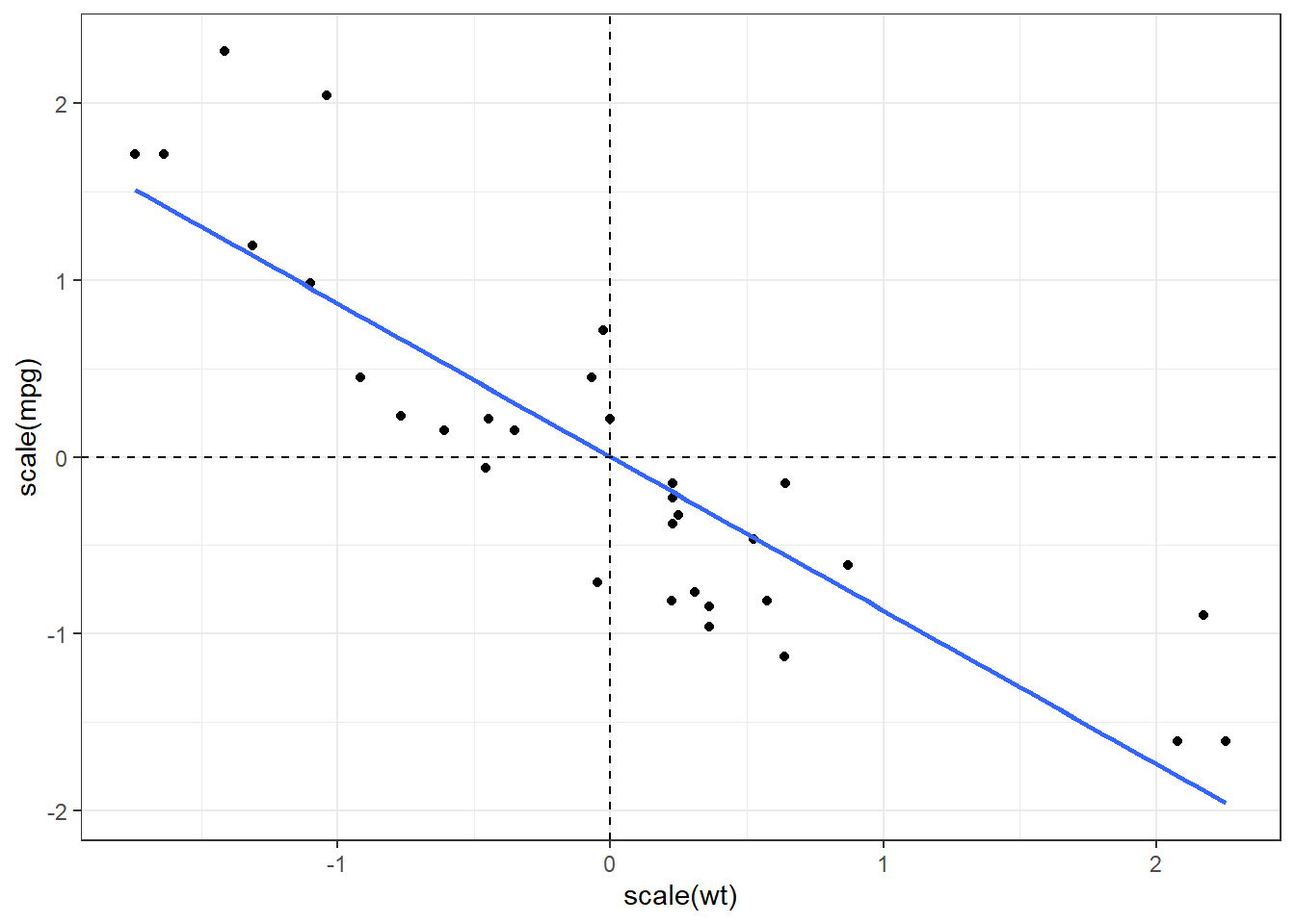
The scale() function scales and center matrix-like objects, such as vectors, using the following formula:
\[ \frac{x_i-\bar{x}}{s_x} \]
The following is the visualization of standardized values in simple linear regression. Notice that the centroid of the scaled x and y variables is (0,0).

We can directly apply this function inside the lm() function to standardize the variables before regression.
##
## Call:
## lm(formula = scale(mpg) ~ scale(wt) + scale(cyl), data = mtcars)
##
## Residuals:
##      Min       1Q   Median       3Q      Max
## -0.71169 -0.25737 -0.07771  0.26120  1.01218
##
## Coefficients:
##               Estimate Std. Error t value Pr(>|t|)
## (Intercept)  4.898e-17  7.531e-02   0.000 1.000000
## scale(wt)   -5.180e-01  1.229e-01  -4.216 0.000222 ***
## scale(cyl)  -4.468e-01  1.229e-01  -3.636 0.001064 **
## ---
## Signif. codes:  0 '***' 0.001 '**' 0.01 '*' 0.05 '.' 0.1 ' ' 1
##
## Residual standard error: 0.426 on 29 degrees of freedom
## Multiple R-squared:  0.8302, Adjusted R-squared:  0.8185
## F-statistic: 70.91 on 2 and 29 DF,  p-value: 6.809e-12
Interpretation: 1 standard deviation increase in weight results to a half standard deviation decrease in miles per gallon.
Exercise 4.10
Standardize the following regression model manually, then estimate the standardized coefficients: \(\hat{y}=50+0.2x_1+3x_2\), where \(s_y=10\), \(s_1=2\), and \(s_2=6\).
Interpret a standardized coefficient of \(\beta^*_3=-0.45\) in terms of standard deviations.
In a multiple regression model that predicts life satisfaction, you find that the standardized coefficient for education is 0.65 and for income is 0.30. Which has a stronger association with life satisfaction, and why?
True or False: Standardizing variables changes the overall model fit (\(R^2\)). Explain your answer.
Relationship to Correlations
Theorem 4.18 If \(\textbf{X}^*\) is a matrix of centered and scaled independent variables, and \(\textbf{Y}^*\) is a vector of centered and scaled dependent variable, then
\[ \frac{1}{n-1}{\textbf{X}^*}^T \textbf{X}^*=\textbf{R}_{xx} \quad \quad \frac{1}{n-1}{\textbf{X}^*}^T \textbf{Y}^*=\textbf{R}_{xy} \]
where \(\textbf{R}_{xx}\) is the correlation matrix of independent variables and \(\textbf{R}_{xy}\) is the correlation vector of the dependent variable with each of the independent variables.
Definition 4.14 A scale invariant least squares estimate of the regression coefficients is given by \[\begin{align} \hat{\boldsymbol{\beta}}^* &= (\textbf{X}^{*T}\textbf{X}^*)^{-1}\textbf{X}^{*T}\textbf{Y}^*\\ &= [(n-1)\textbf{R}_{xx}]^{-1}[(n-1)\textbf{R}_{xy}] \end{align}\]
Exercise 4.11 In this exercise, we visualize Theorem 4.18 using actual data. Let’s try mtcars, where the dependent variable ismpg, and the independent variables are the rest. Follow these steps in R.
Split the dataframe into vector of dependent variables \(\textbf{Y}\) and matrix of independent variables \(\textbf{X}\).
Y <- as.matrix(mtcars[,1])X <- as.matrix(mtcars[,2:11])
Scale and center all \(\textbf{Y}\) and \(\textbf{X}\) to \(\textbf{Y}^*\) and \(\textbf{X}^*\) respectively. The
scalefunction may help in transforming a matrix per column.Perform the matrix operations \(\frac{1}{n-1}{\textbf{X}^*}^T\textbf{X}^*\) and \(\frac{1}{n-1}{\textbf{X}^*}^T\textbf{Y}^*\)
Obtain correlations \(\textbf{R}_{xx}\) and \(\textbf{R}_{xy}\). You may use the functions
cor(X)andcor(X,Y)respectively.
What can you say about the results of 3 and 4?