Chapter 2 Law Firm Analysis
2.1 Introduction
The purpose of this chapter was to examine data about violations and tickets among different states such as NY, NJ, and CT. I analyzed the data to answer questions such as whether certain counties have higher payment amounts, if certain agencies issue higher payments, and if drivers from different states pay different amounts for tickets.
2.3 Overview
I’m a data scientist, currently working for a Law Firm that specializes in fighting parking and camera tickets. They want me to uncover hidden patterns in NYC violation data such as:
If certain agencies issue higher payments?
If drivers from different states (NY, NJ, CT) pay more?
If certain counties tend to have higher payment amounts?
I will be using and analyzing NYC violation data from NYCOpenData, which can be found at this link: https://data.cityofnewyork.us/City-Government/Open-Parking-and-Camera-Violations/nc67-uf89/about_data
2.4 Agency
ggplot(camera, aes(x = issuing_agency, y = payment_amount)) + geom_boxplot() + labs(
  title= "Agency and Payment Amount",
  x = "Agency",
  y = "Payment Amount")+ theme_minimal() + coord_flip()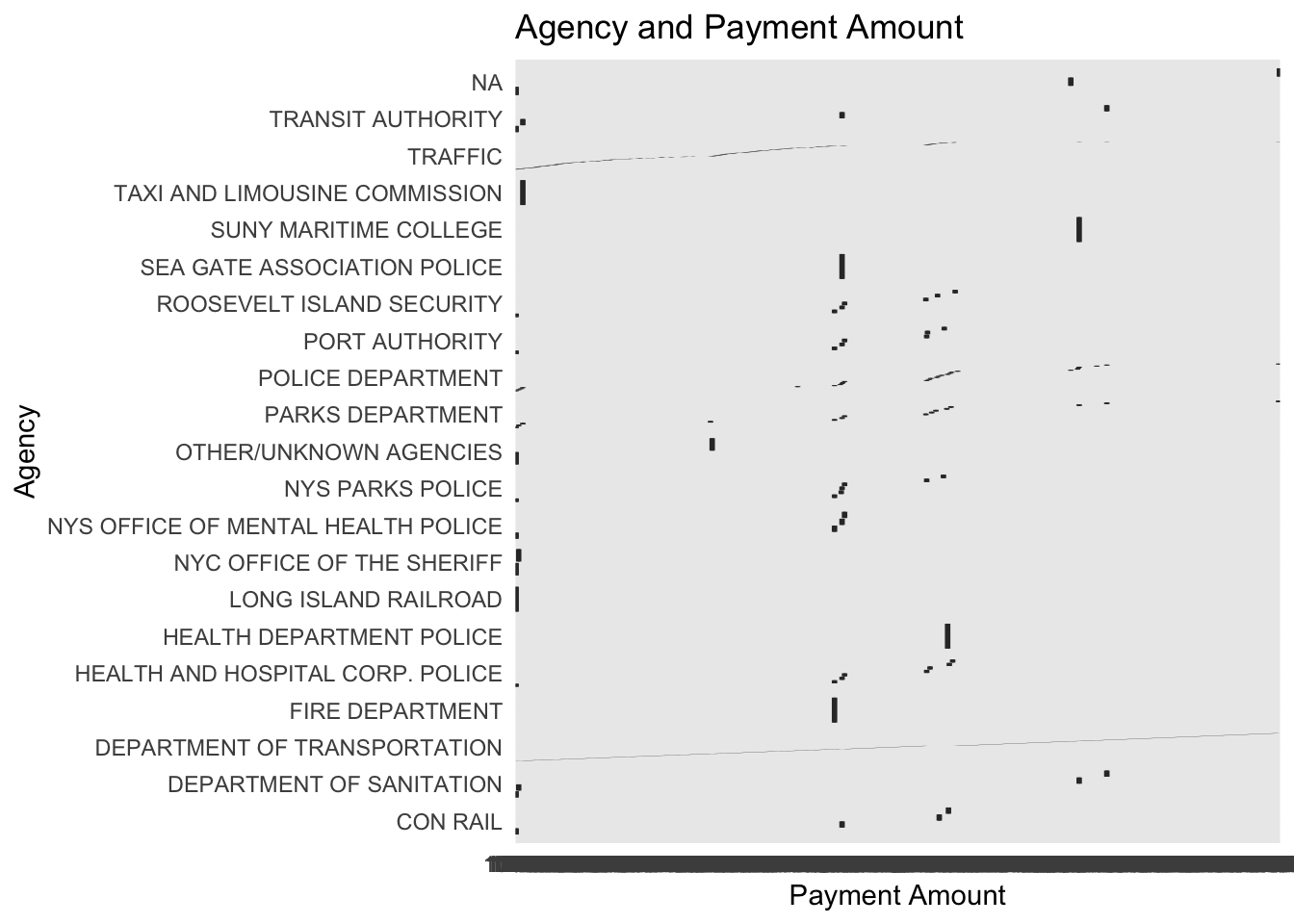
Figure 2.1: This is supposed to be a boxplot showing the different payment amounts across groups.
##                        issuing_agency    min      Q1 median       Q3    max      mean        sd     n missing
## 1            HEALTH DEPARTMENT POLICE 243.81 243.810 243.81 243.8100 243.81 243.81000        NA     1       0
## 2         SEA GATE ASSOCIATION POLICE 190.00 190.000 190.00 190.0000 190.00 190.00000   0.00000     2       0
## 3                     FIRE DEPARTMENT 180.00 180.000 180.00 180.0000 180.00 180.00000        NA     1       0
## 4  NYS OFFICE OF MENTAL HEALTH POLICE   0.00 180.000 180.00 190.0000 210.00 161.33333  65.99423    15       0
## 5           ROOSEVELT ISLAND SECURITY   0.00 135.000 180.00 190.0000 246.68 149.16083  90.57967    24       0
## 6                      PORT AUTHORITY   0.00 180.000 180.00 190.0000 242.76 147.35792  82.58394    48       0
## 7                    NYS PARKS POLICE   0.00  45.000 180.00 190.0000 242.58 143.86176  89.24158    34       0
## 8                    PARKS DEPARTMENT   0.00  90.000 180.00 190.0000 245.28 128.47736  78.92728   144       0
## 9       TAXI AND LIMOUSINE COMMISSION 125.00 125.000 125.00 125.0000 125.00 125.00000        NA     1       0
## 10   HEALTH AND HOSPITAL CORP. POLICE   0.00   0.000 180.00 190.0000 245.64 124.71373  98.60130    51       0
## 11                  POLICE DEPARTMENT   0.00   0.000 180.00 190.0000 260.00 123.93855  88.00388   214       0
## 12                           CON RAIL   0.00   0.000  95.00 228.8875 243.87 112.62000 124.87146     6       0
## 13       DEPARTMENT OF TRANSPORTATION   0.00  50.000  75.00 125.0000 690.04  99.52822  82.88394 87273       0
## 14                            TRAFFIC   0.00  65.000 115.00 115.0000 245.79  94.59362  44.47453 12091       0
## 15             OTHER/UNKNOWN AGENCIES   0.00  40.115  80.23 120.3450 160.46  80.23000 113.46235     2       0
## 16                  TRANSIT AUTHORITY   0.00   0.000  75.00 125.0000 190.00  78.00000  82.05181     5       0
## 17              SUNY MARITIME COLLEGE  65.00  65.000  65.00  65.0000  65.00  65.00000        NA     1       0
## 18          NYC OFFICE OF THE SHERIFF   0.00  28.750  57.50  86.2500 115.00  57.50000  81.31728     2       0
## 19           DEPARTMENT OF SANITATION   0.00   0.000  65.00 105.0000 115.00  56.78571  48.26239    14       0
## 20 LONG ISLAND RAILROAD 0.00 0.000 0.00 0.0000 0.00 0.00000 NA 1 0## Df Sum Sq Mean Sq F value Pr(>F)
## issuing_agency 19 937675 49351 7.858 <2e-16 ***
## Residuals 99910 627464684 6280
## ---
## Signif. codes: 0 '***' 0.001 '**' 0.01 '*' 0.05 '.' 0.1 ' ' 1
## 69 observations deleted due to missingness## Analysis of Variance Table (Type III SS)
## Model: payment_amount ~ issuing_agency
##
## SS df MS F PRE p
## ----- --------------- | ------------- ----- --------- ----- ----- -----
## Model (error reduced) | 937675.432 19 49351.339 7.858 .0015 .0000
## Error (from model) | 627464683.951 99910 6280.299
## ----- --------------- | ------------- ----- --------- ----- ----- -----
## Total (empty model) | 628402359.383 99929 6288.488** Interpretation**
In our findings, when looking at the sum of squares, we can see that there is a small amount of variance related to the issuing agency. The F-value (7.858) is pretty small, and the p-value (<2e-16) conveys that the difference is statistically significant. 0.15% of the variance is explained, conveying how little of the variation in payment amount is related to the issuing agency. I would not recommend the law firm to use the issuing agency in their marketing strategy because of how small the variation and f-value is.
2.5 Plate State
ggplot(camera, aes(x = state, y = payment_amount)) + geom_boxplot() + labs(
  title= "Plate State and Payment Amount",
  x = "State",
  y = "Payment Amount")+ theme_minimal() + coord_flip()
Figure 2.2: This is supposed to be a boxplot that shows the plate states and their payment amounts.
##    state    min     Q1 median       Q3    max      mean        sd     n missing
## 1     OK   0.00  50.00 200.00 250.0000 250.00 162.19719 88.522638   160       0
## 2     ON 115.00 115.00 120.00 130.0000 145.00 125.00000 14.142136     4       0
## 3     QB 115.00 115.00 115.00 125.0000 125.00 118.75000  5.175492     8       0
## 4     NB 115.00 115.00 115.00 115.0000 115.00 115.00000        NA     1       0
## 5     AR  50.00  50.00 100.00 150.0000 250.00 113.30731 72.563803    67       0
## 6     WA   0.00  50.00  50.00 125.0000 275.00 109.09091 92.114522    33       0
## 7     TX   0.00  50.00  75.04 126.4025 277.06 104.12010 69.855661   312       0
## 8     DC  50.00  75.43 115.00 117.6800 145.00 102.66700 29.610797    20       0
## 9     NJ   0.00  50.00  75.00 115.0000 682.35 101.57462 89.971702  8654       3
## 10    NY   0.00  50.00  75.00 125.0000 690.04 101.09015 80.930148 79541      10
## 11    IN   0.00  67.50 115.00 115.0000 250.00  99.16667 50.520663    42       0
## 12    MN   0.00  50.00  75.00 107.5000 250.00  91.05847 68.580471    59       0
## 13    OH   0.00  50.00  75.00 115.0000 281.80  90.77151 65.548205   299       0
## 14    MT  50.00  50.00  87.50 100.0000 225.00  90.62500 43.671513    24       0
## 15    AL   0.00  50.00  75.00 115.0000 277.06  89.53567 56.218191    97       0
## 16    NC   0.00  50.00  75.00 115.0000 275.89  88.74886 57.680647   484       1
## 17    IL   0.00  50.00  75.00 100.0000 275.00  86.22200 54.900047   265       0
## 18    PA   0.00  50.00  75.00 100.0000 283.57  85.92090 53.933428  2977       2
## 19    IA  50.00  50.00  75.00  93.7600 175.00  85.00400 44.408710    10       0
## 20    VA   0.00  50.00  50.00 115.0000 275.00  82.70679 53.216823   527       0
## 21    SC   0.00  50.00  75.02 100.0000 250.00  82.61794 41.265398   194       0
## 22    GA   0.00  50.00  50.00 100.0000 275.62  82.57126 63.360707   302       0
## 23    MD   0.00  50.00  50.00 100.0000 250.00  81.02126 46.705884   413       0
## 24    CT   0.00  50.00  75.00 100.0000 276.57  80.66270 46.078493  1457       2
## 25    DE   0.00  50.00  75.00  75.4625 275.00  79.71512 49.576008    84       1
## 26    FL   0.00  50.00  50.00 100.0000 276.10  79.26281 50.883529  1654       2
## 27    AZ   0.00  50.00  50.00 100.0000 250.00  79.14683 50.917069   556       0
## 28    MO   0.00  50.00  50.00  75.1900 250.00  78.81636 57.999183    33       0
## 29    MA   0.00  50.00  50.00 100.0000 278.02  78.02744 48.262245   735       0
## 30    VT   0.00  50.00  75.00  75.7550 200.00  77.40515 41.129903    68       0
## 31    MS   0.00  50.00  75.16 115.0000 125.87  76.78111 42.988707     9       0
## 32    AK  75.95  75.95  75.95  75.9500  75.95  75.95000        NA     1       0
## 33    NH  50.00  50.00  50.00 100.0000 178.39  75.04704 31.790066    54       0
## 34    LA  50.00  50.00  50.00  76.4375 241.31  73.36333 41.807692    24       0
## 35    CA   0.00  50.00  50.00 100.0000 275.00  73.04461 52.607199   128       0
## 36    WI   0.00  50.00  50.00 115.0000 125.00  70.62500 44.460840    24       0
## 37    ME   0.00  50.00  50.00  75.4950 250.00  69.10433 37.054284    67       0
## 38    MI   0.00  50.00  50.00  75.0300 225.06  68.87076 35.774572   118       1
## 39    RI   0.00  50.00  50.00  75.5925 241.36  68.77096 36.502474   104       0
## 40    WV  50.00  50.00  50.00  75.6900 125.72  66.91444 25.274199     9       0
## 41    NV  50.00  50.00  50.00  75.0000 125.00  66.47059 26.325172    17       0
## 42    TN  50.00  50.00  50.00  75.0000 180.00  66.27884 30.075361    95       0
## 43    NE   0.00  50.00  50.00  85.0000 180.00  66.25000 51.527795    12       0
## 44    CO   0.00  50.00  50.00  75.0000 125.00  64.51613 28.992954    31       0
## 45    KY  50.00  50.00  50.00  75.0000 125.00  63.41818 25.188157    33       0
## 46    OR  50.00  50.00  50.00  61.2500 125.00  63.01793 23.969258    58       0
## 47    NM  50.00  50.00  50.00  63.1050  76.21  58.73667 15.132351     3       0
## 48    SD   0.00  50.00  62.50  75.0000 125.00  55.36929 35.604580    14       0
## 49    KS   0.00  12.50  50.00  87.5000 115.00  52.50000 48.347699     6       0
## 50    ID  50.00  50.00  50.00  50.0000  50.00  50.00000        NA     1       0
## 51    ND  50.00  50.00  50.00  50.0000  50.00  50.00000        NA     1       0
## 52    DP   0.00   0.00   0.00 115.0000 115.00  49.28571 61.470086     7       0
## 53    UT   0.00  50.00  50.00  50.0000  50.00  38.88889 22.047928     9       0
## 54 99 0.00 0.00 0.00 0.0000 190.00 20.51724 46.605196 29 43## Df Sum Sq Mean Sq F value Pr(>F)
## state 53 4867057 91831 14.71 <2e-16 ***
## Residuals 99880 623567686 6243
## ---
## Signif. codes: 0 '***' 0.001 '**' 0.01 '*' 0.05 '.' 0.1 ' ' 1
## 65 observations deleted due to missingness## Analysis of Variance Table (Type III SS)
## Model: payment_amount ~ state
##
## SS df MS F PRE p
## ----- --------------- | ------------- ----- --------- ------ ----- -----
## Model (error reduced) | 4867056.569 53 91831.256 14.709 .0077 .0000
## Error (from model) | 623567685.704 99880 6243.169
## ----- --------------- | ------------- ----- --------- ------ ----- -----
## Total (empty model) | 628434742.273 99933 6288.5612.6 Interpretation
In our findings, when looking at the sum of squares, we can see that there is a small amount of variance related to the different states. The F-value (14.709) is small, and the p-value (<2e-16) conveys that the difference is statistically significant. 0.77% of the variance is explained, conveying how little of the variation in payment amount is related to the different states. I would not recommend the law firm to use states in their marketing strategy because of how small the variation and f-value is, even though it is statistically significant.
2.7 County
camera<- camera %>%
  mutate(
    county_clean= str_replace(county, "Q", "Queens County"),
    county_clean= str_replace(county_clean, "K", "Kings County")
)ggplot(camera, aes(x = county_clean, y = payment_amount)) + geom_boxplot() + labs(
title= "County and Payment Amount",
x = "County",
y = "Payment Amount")+ theme_minimal() + coord_flip()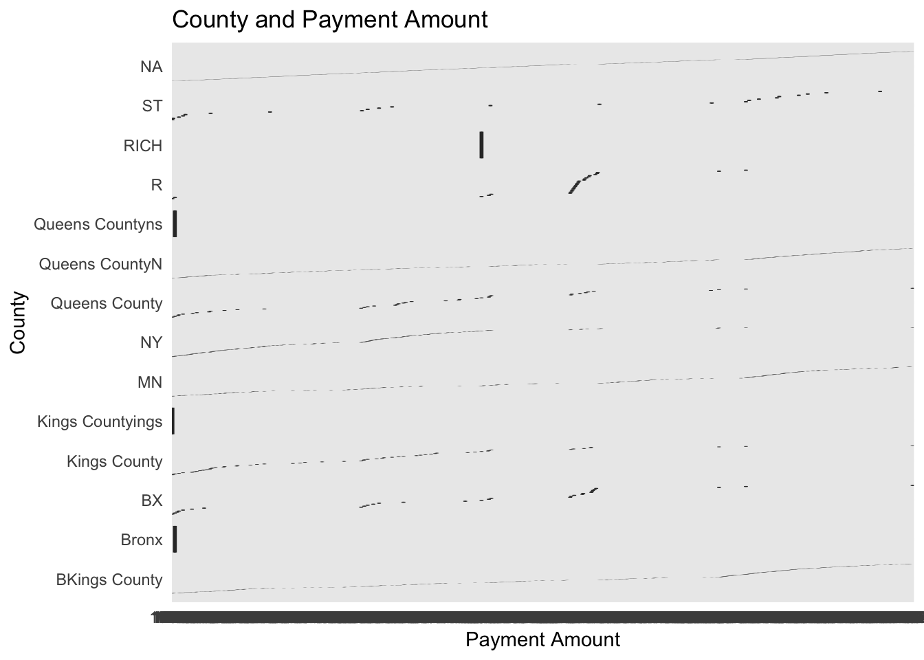
Figure 2.3: This is supposed to be a boxplot showing the different payment amounts across counties.
##        county_clean min  Q1 median     Q3    max      mean        sd     n missing
## 1              RICH 180 180    180 180.00 180.00 180.00000        NA     1       0
## 2                 R   0  65    180 180.00 245.79 139.67920  80.35405   863       0
## 3             Bronx 115 115    115 115.00 115.00 115.00000        NA     1       0
## 4   Queens Countyns 115 115    115 115.00 115.00 115.00000        NA     1       0
## 5     BKings County   0  50     75 100.00 690.04 113.54971 131.50278 14560       0
## 6     Queens County   0  65    115 125.00 244.46 101.70729  53.07962   992       0
## 7                MN   0  50     50 125.06 281.80 100.54274  73.46670 14518       0
## 8                BX   0  65     75 145.00 245.64  99.59634  67.66429   246       0
## 9                NY   0  65    115 115.00 260.00  92.89794  38.39107  8961       0
## 10     Kings County   0  65     65 115.00 243.81  85.99174  49.27722  1551       0
## 11   Queens CountyN   0  50     50 100.00 283.03  82.35782  60.30923 16373       0
## 12               ST   0  50     50  75.00 250.00  69.66361  45.80596   485       0
## 13 Kings Countyings 0 0 0 0.00 0.00 0.00000 NA 1 0## Df Sum Sq Mean Sq F value Pr(>F)
## county_clean 12 9980943 831745 116.7 <2e-16 ***
## Residuals 58540 417135006 7126
## ---
## Signif. codes: 0 '***' 0.001 '**' 0.01 '*' 0.05 '.' 0.1 ' ' 1
## 41446 observations deleted due to missingness## Analysis of Variance Table (Type III SS)
## Model: payment_amount ~ county_clean
##
## SS df MS F PRE p
## ----- --------------- | ------------- ----- ---------- ------- ----- -----
## Model (error reduced) | 9980942.982 12 831745.249 116.726 .0234 .0000
## Error (from model) | 417135005.877 58540 7125.641
## ----- --------------- | ------------- ----- ---------- ------- ----- -----
## Total (empty model) | 427115948.859 58552 7294.643** Interpretation paragraph**
In our findings, when looking at the sum of squares, we can see that there is a small amount of variance related to the different counties. The F-value (116.726) is large, and the p-value (<2e-16) conveys that the difference is statistically significant. 2.34% of the variance is explained, conveying that there is some variation in payment amount that is related to the the different counties. I would recommend the law firm to use the the different counties in their marketing strategy because of the large F-value as well as the variance that is related to payment amount.
2.8 Final
I think that the firm should prioritize the different counties in its marketing efforts. The reason is because out of the 3 variables (agency, state, and county), county is the variable that has the largest f-value, as well as the most variation that is related to payment amount compared to the other 2 variables.