Chapter 4 NBA Analytics
4.1 Introduction
The purpose of this chapter was to examine if there is a relationship between west and east coast teams. looked at some stats from teams such as point, rebounds, assists, steals, and blocks and examined if there were any correlations between east and west coast teams.
4.2 Loading and Preparing the Data
library(readxl)
library(tidyverse)
NBA_teams<- read_xlsx("NBA Team Total Data 2024-2025.xlsx")
View(NBA_teams)

loading_teams<- function(file_name,team_name,sheet_name,PRA, Stocks){
  team_data<- read_xlsx(file_name, sheet=sheet_name)
  team_data$Team<- team_name
  team_data$Sheet<- sheet_name
  team_data$PRA<- rowSums(team_data[, c("PTS", "ORB", "AST")], na.rm=TRUE)
  team_data$Stocks<- rowSums(team_data[, c("STL", "BLK")], na.rm=TRUE)
  team_data$Won_award<-ifelse(is.na(team_data$Awards),"0","1")
  return(team_data)
}
team_warrior<- loading_teams("NBA Team Total Data 2024-2025.xlsx", "Warriors", "Warriors", "PRA", "Stocks")
team_warrior
## # A tibble: 23 × 35
## Rk Player Age G GS MP FG FGA `FG%` `3P` `3PA` `3P%` `2P` `2PA` `2P%` `eFG%` FT FTA
## <dbl> <chr> <dbl> <dbl> <dbl> <dbl> <dbl> <dbl> <dbl> <dbl> <dbl> <dbl> <dbl> <dbl> <dbl> <dbl> <dbl> <dbl>
## 1 1 Stephe… 36 70 70 2252 564 1258 0.448 311 784 0.397 253 474 0.534 0.572 279 299
## 2 2 Draymo… 34 68 66 1983 216 509 0.424 80 246 0.325 136 263 0.517 0.503 101 147
## 3 3 Buddy … 32 82 22 1863 328 786 0.417 203 549 0.37 125 237 0.527 0.546 53 64
## 4 4 Brandi… 21 64 33 1716 280 629 0.445 115 309 0.372 165 320 0.516 0.537 72 95
## 5 5 Moses … 22 74 34 1649 246 568 0.433 126 337 0.374 120 231 0.519 0.544 106 133
## 6 6 Andrew… 29 43 43 1296 261 588 0.444 94 248 0.379 167 340 0.491 0.524 139 179
## 7 7 Jonath… 22 47 10 1144 258 568 0.454 46 151 0.305 212 417 0.508 0.495 157 235
## 8 8 Kevon … 28 76 6 1142 143 278 0.514 2 5 0.4 141 273 0.516 0.518 56 99
## 9 9 Jimmy … 35 30 30 980 159 334 0.476 19 68 0.279 140 266 0.526 0.504 201 231
## 10 10 Trayce… 24 62 37 967 174 302 0.576 0 3 0 174 299 0.582 0.576 59 102
## # ℹ 13 more rows
## # ℹ 17 more variables: `FT%` <dbl>, ORB <dbl>, DRB <dbl>, TRB <dbl>, AST <dbl>, STL <dbl>, BLK <dbl>, TOV <dbl>,
## # PF <dbl>, PTS <dbl>, `Trp-Dbl` <dbl>, Awards <chr>, Team <chr>, Sheet <chr>, PRA <dbl>, Stocks <dbl>,
## # Won_award <chr>## [1] "/Users/crystaladote/Downloads/Reproducible Psyc Fall 2025/Bookdown_assignment"path<- "/Users/crystaladote/Downloads/Reproducible Psyc Fall 2025/NBA Team Total Data 2024-2025.xlsx"
file.exists(path)## [1] TRUE## [1] "Nets" "Knicks" "Raptors" "Philly" "Celtics" "Timberwolves" "Thunder"
## [8] "Jazz" "Trailblazers" "Nuggets" "Bulls" "Bucks" "Cavaliers" "Pistons"
## [15] "Pacers" "Warriors" "Suns" "Lakers" "Clippers" "Kings" "Hornets"
## [22] "Magic" "Wizards" "Hawks" "Heat" "Grizzles" "Spurs" "Pelicans"
## [29] "Rockets" "Mavericks"file_name <- "/Users/crystaladote/Downloads/Reproducible Psyc Fall 2025/NBA Team Total Data 2024-2025.xlsx"
team_sheets <- excel_sheets(file_name)
all_teams <- bind_rows(
lapply(team_sheets, function(sheet_name) {
loading_teams(file_name = file_name, team_name = sheet_name, sheet_name = sheet_name)
})
)
View(all_teams)4.4 Visual Exploration
library(ggplot2)
ggplot(full_team_data, aes(x=PRA, y=Stocks, color=Conference))+
  geom_point()+
  labs(
    title= "Relationship between PRA and Stocks",
    x= "PRA",
    y= "Stocks"
  )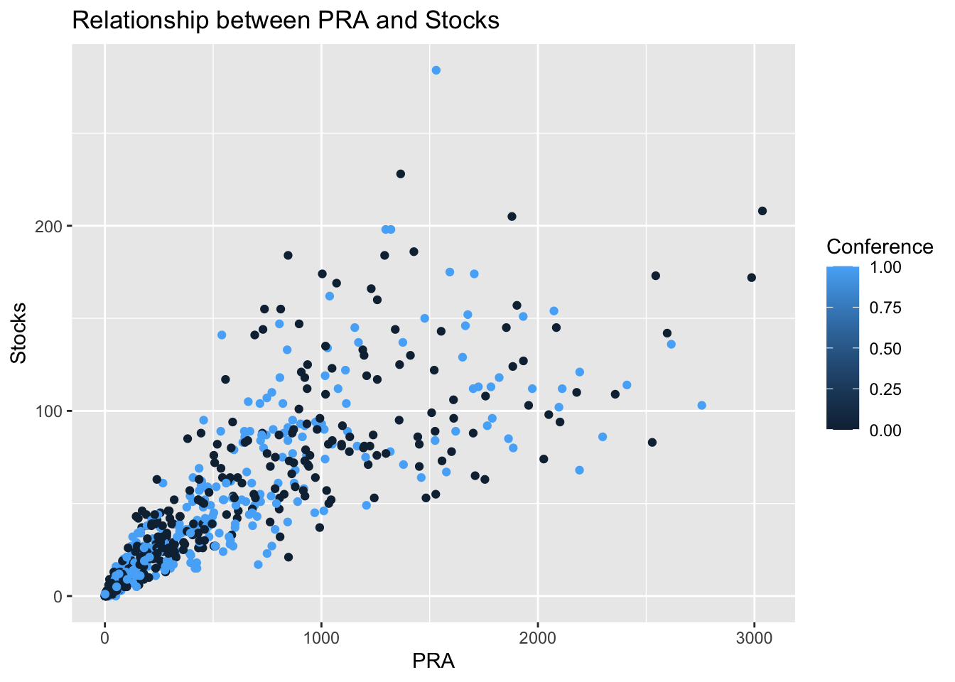
Figure 4.1: This scatter plot shows us the relationship between PRA and Stocks.
This scatter plot shows us that for both conferences (East and West), there is a positive relationship between PRA and Stocks.
ggplot(full_team_data, aes(x=DRB, y=STL, color= Conference)) +
  geom_point()+
  labs(
    title= "Relationship between Defensive Rebounds and Steals",
    x= "Defensive Rebounds",
    y= "Steals"
  )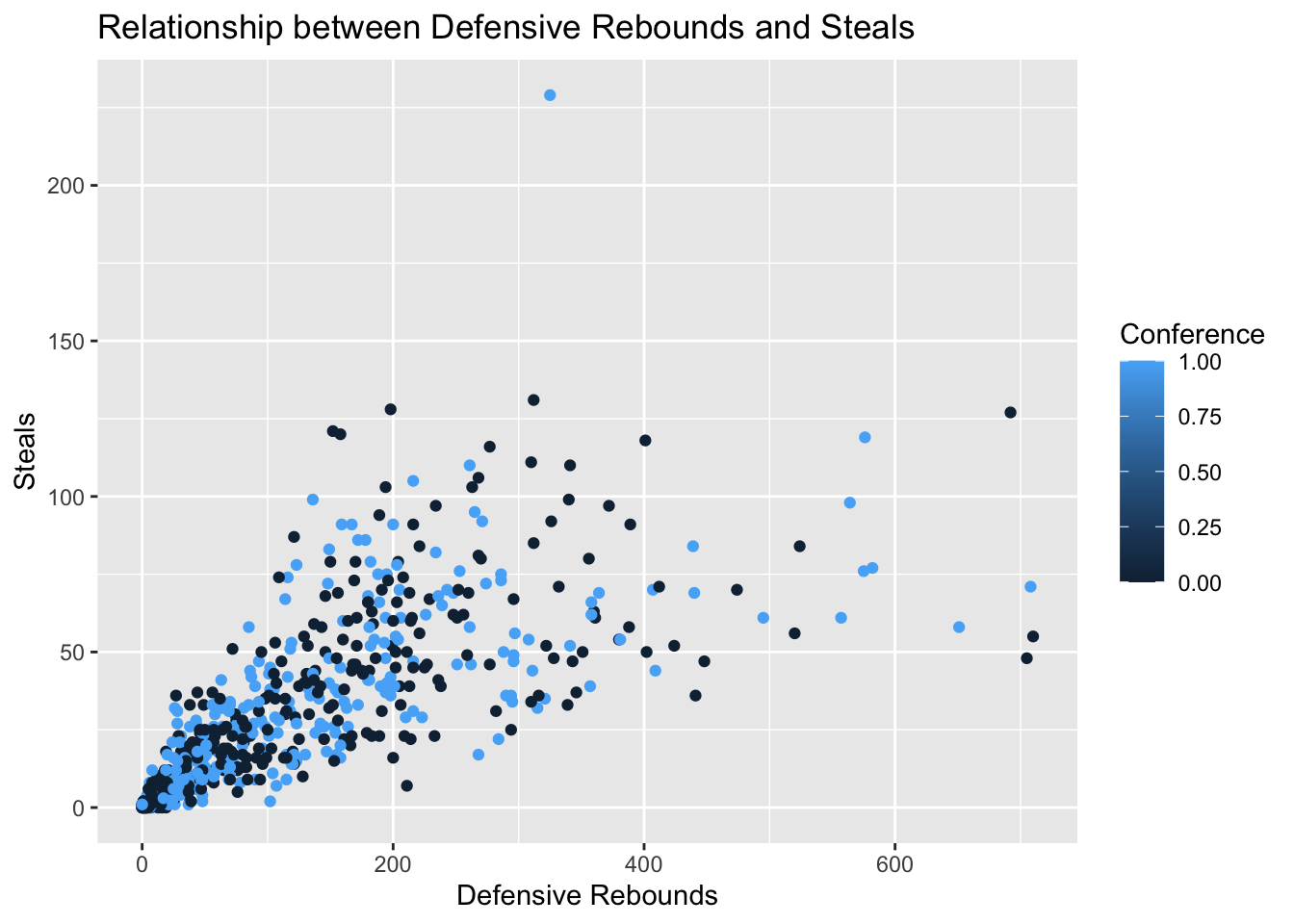
Figure 4.2: This scatter plot shows the relationship between defensive rebounds and steals.
The scatter plot shows us that there is a positive relationship with defensive rebounds and steals for both East and West.
4.5 Correlation Analysis
##
##  Pearson's product-moment correlation
##
## data:  x and y
## t = -1.7941, df = 650, p-value = 0.07325
## alternative hypothesis: true correlation is not equal to 0
## 95 percent confidence interval:
##  -0.146194514  0.006620927
## sample estimates:
##         cor
## -0.07019864
There is a negative, weak correlation between PRA and Conference (-0.070). This correlation is not statistically significant, given that it has a p-value of 0.073.
##
##  Pearson's product-moment correlation
##
## data:  x and y
## t = -2.094, df = 650, p-value = 0.03665
## alternative hypothesis: true correlation is not equal to 0
## 95 percent confidence interval:
##  -0.157650363 -0.005105577
## sample estimates:
##         cor
## -0.08185737
There is a negative,weak correlation between Stocks and Conference (-0.0818). However, this correlation is statistically significant, with a p-value of 0.036.
library(ggcorrplot)
stats_matrix<- full_team_data %>% dplyr::select(Age, PRA, Stocks)
APS_matrix<- cor(stats_matrix, use="pairwise.complete.obs")
APS_matrix
## Age PRA Stocks
## Age 1.00000000 0.1246811 0.07734898
## PRA 0.12468112 1.0000000 0.81779753
## Stocks 0.07734898 0.8177975 1.00000000ggcorrplot(APS_matrix, lab=TRUE, type="lower")+
labs(title="Correlation Matrix: Age, PRA, and Stocks")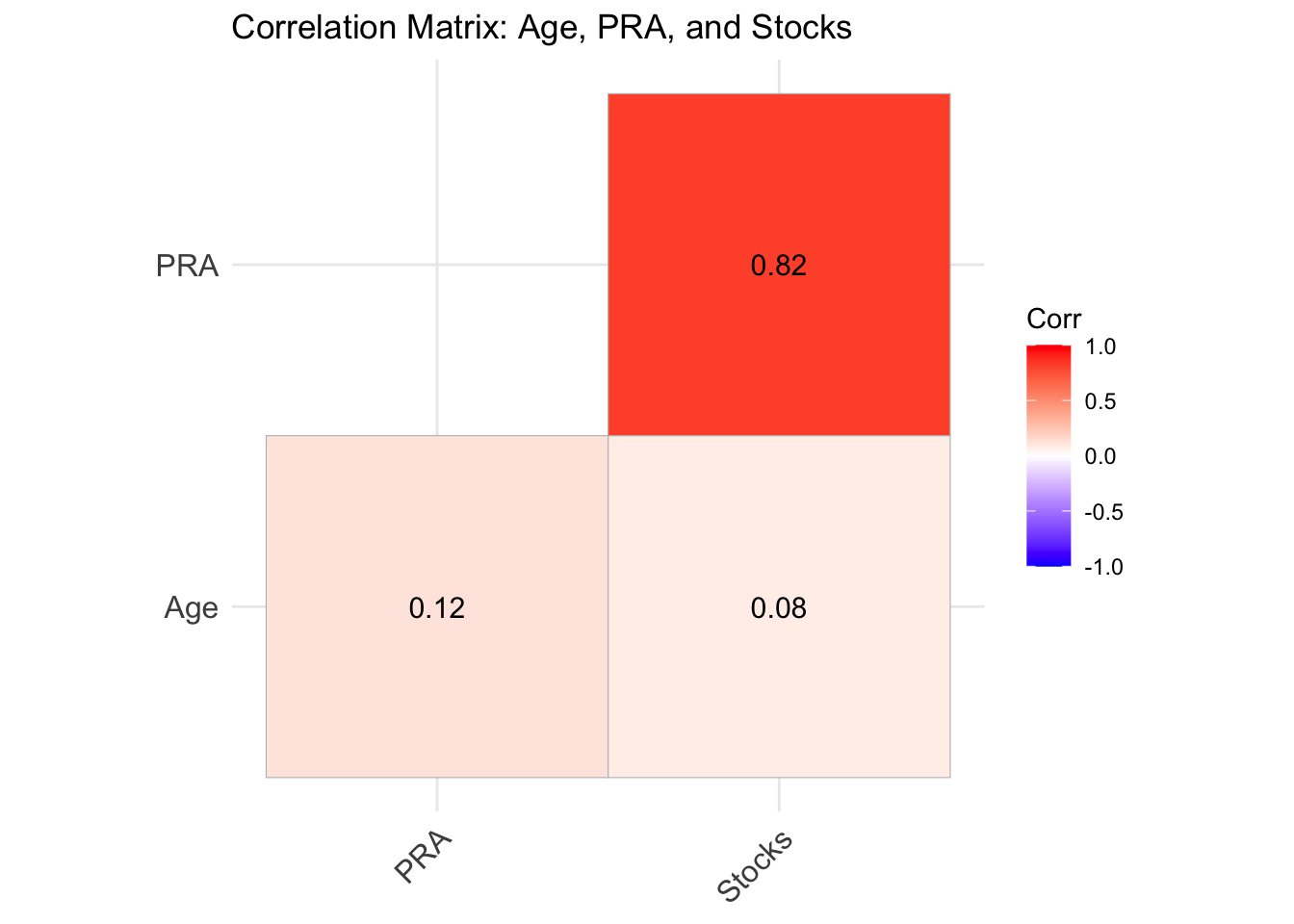
Figure 4.3: This figure looks at the correlation matrix that includes age, PRA, and Stocks.
The relationship between PRA and Stocks is the strongest, with a positive correlation of 0.82. It is the closest out of all 3 correlations to 1.
##    estimate       p.value statistic   n gp  Method
## 1 0.8169568 2.748291e-157   36.0888 652  1 pearson
Controlling for the variable Age conveys that there is a strong positive correlation between PRA and Stocks (0.81695). Meaning that age doesn’t much effect on those 2 variables. It also shows us that it is statistically significant due to the p-value.
4.6 Findings
To Mr. Silver,
According to the findings, and correlations there doesn’t appear to be a difference between the East and West teams, especially regarding PRA (points, rebounds, and assists) and Stocks (steals and blocks). We also saw that there is a strong, positive correlation between PRA and Stocks when Age was controlled, conveying that age doesn’t have an effect on either variables. One scatter plot showed the relationship between defensive rebounds and steals conveying that offensive and defensive performances tend to move together. The scatter plot conveys a positive, somewhat strong correlation between the two variables. One potential next step for when analyzing this data could be to look at the relationship between the 2-point and 3-point averages and possibly field goal average. One limitation of my analysis would be that the weak correlations that were observed could possibly be due to other factors that aren’t in the data.