7  Orthogonality

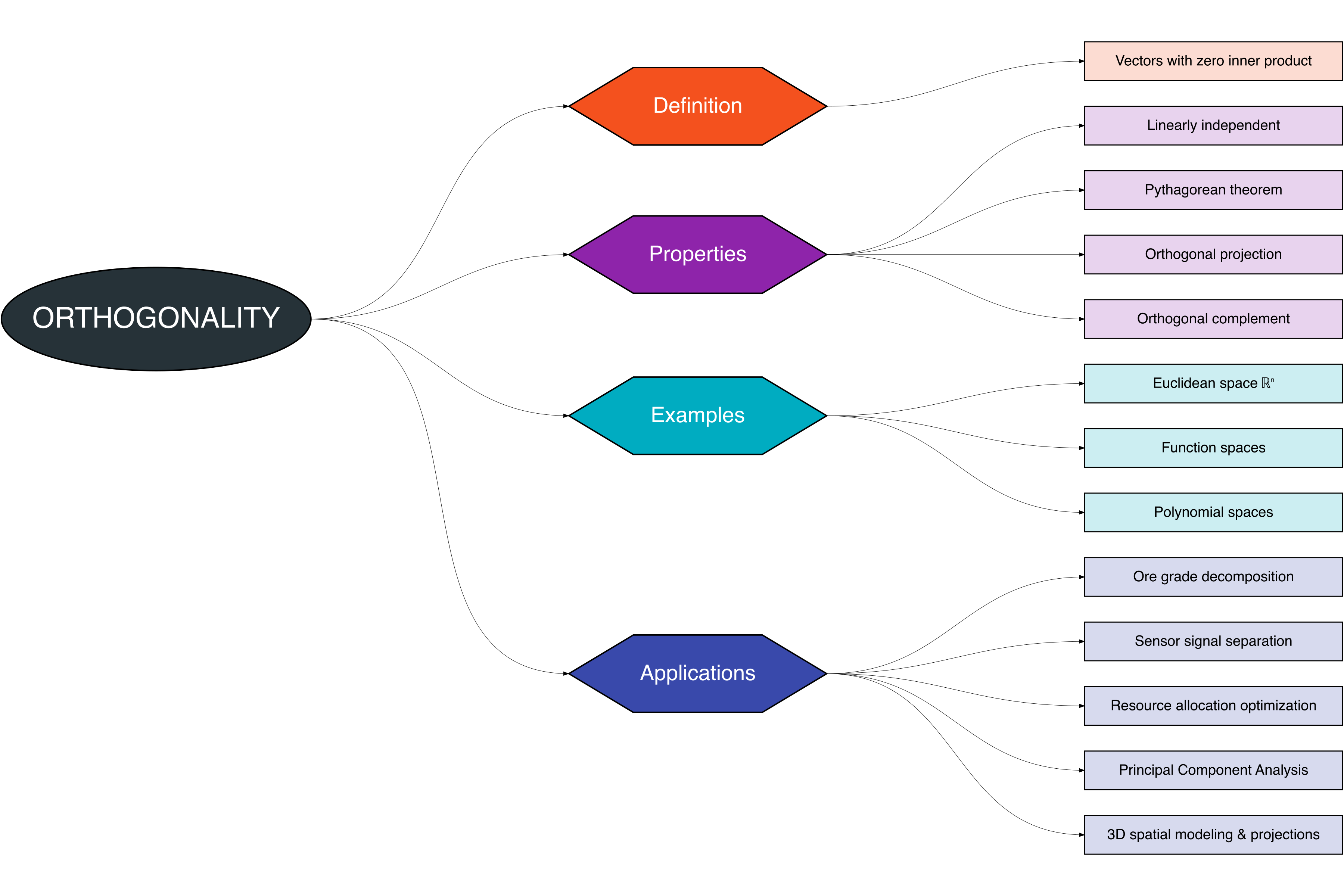
In this chapter, we explore the concept of orthogonality in vector and inner product spaces, along with its fundamental properties. A mind map provides a structured overview of the key topics discussed:

Figure 7.1: Mind Map of Orthogonality in Inner Product Spaces

Orthogonality is a key concept in inner product spaces, describing vectors that are perpendicular to each other. Two vectors \(u\) and \(v\) are orthogonal if their inner product satisfies \(u \cdot v = 0\). Orthogonal vectors provide a framework for decomposition, projections, and simplification of vector representations.

In the context of mining engineering:

• Ore Classification: Different ore samples can be represented as vectors in \(\mathbb{R}^n\). Orthogonal vectors indicate uncorrelated ore characteristics, which is useful for separating ore types or creating independent quality indices chiles2012?.
  
• Sensor Data Decorrelation: Sensor measurements across mine sites can be transformed into orthogonal components to reduce redundancy and highlight independent signal features, aiding in anomaly detection and predictive maintenance [1].
  
• Projection for Resource Optimization: Tasks such as workforce or equipment assignment can be projected onto orthogonal directions to isolate independent effects, supporting least-squares optimization and operational efficiency meyer2000?.
  
• Geostatistical Modeling: Spatial data vectors can be decomposed into orthogonal components, facilitating kriging, spatial variance analysis, and reducing multicollinearity in predictive models rubinstein2016?.
  
• 3D Spatial Planning: Orthogonality in \(\mathbb{R}^3\) helps in tunnel design, shaft alignment, and modeling ore body orientations, ensuring minimal interference and accurate geometric calculations chiles2012?.

Orthogonality provides a robust tool for simplifying complex vector interactions, enabling decomposition, projection, and independent analysis. This is essential for optimization, geostatistical modeling, and operational planning in mining, extending the analytical capabilities of inner product spaces [1], meyer2000?, chiles2012?, rubinstein2016?.

7.1 Definition

Two vectors \(u\) and \(v\) in an inner product space \(V\) are orthogonal if their inner product is zero:

\[ \langle u, v \rangle = 0 \]

Key points:

• Orthogonal vectors are “perpendicular” in a generalized sense.
• Orthogonality extends to sets of vectors: a set \(\{v_1, v_2, \dots, v_n\}\) is orthogonal if \(\langle v_i, v_j \rangle = 0\) for \(i \neq j\).
• If additionally \(\|v_i\| = 1\), the set is orthonormal.

7.2 Properties

• Pythagorean Theorem:
  If \(u \perp v\), then
  \[ \|u + v\|^2 = \|u\|^2 + \|v\|^2 \]

• Linear Independence:
  Nonzero orthogonal vectors are linearly independent.

• Projection:
  The orthogonal projection of \(u\) onto \(v\) is
  \[ \text{proj}_v(u) = \frac{\langle u, v \rangle}{\langle v, v \rangle} v \]

• Orthogonal Complement:
  For a subspace \(W \subset V\),
  \[ W^\perp = \{v \in V : \langle v, w \rangle = 0, \forall w \in W\} \]

7.3 Examples

1. Euclidean space \(\mathbb{R}^2\) or \(\mathbb{R}^3\)
   Standard basis vectors are orthogonal:
   \[ e_1 = \begin{bmatrix}1 \\ 0 \\ 0\end{bmatrix}, e_2 = \begin{bmatrix}0 \\ 1 \\ 0\end{bmatrix}, e_3 = \begin{bmatrix}0 \\ 0 \\ 1\end{bmatrix} \]

2. Function space \(L^2[a,b]\)
   Functions \(f\) and \(g\) are orthogonal if
   \[ \int_a^b f(x) g(x) dx = 0 \]

3. Polynomial space
   Polynomials \(p_i(x)\) and \(p_j(x)\) can be orthogonal under a weighted inner product
   \[ \langle p_i, p_j \rangle = \int_a^b p_i(x) p_j(x) w(x) dx = 0 \]

7.4 Applications

• Ore Grade Decomposition:
  Orthogonal vectors can represent independent ore grade variations. This allows separation of correlated and uncorrelated components in ore modeling chiles2012?.

• Signal Processing / Sensor Analysis:
  Orthogonal signals reduce interference and enable independent feature extraction from geotechnical or seismic sensors [1].

• Resource Allocation Optimization:
  Using orthogonal vectors in task allocation ensures non-overlapping responsibilities, minimizing redundancy in equipment or workforce assignments meyer2000?.

• 3D Spatial Modeling:
  Orthogonal basis vectors in \(\mathbb{R}^3\) support coordinate transformations, visualization of tunnels, boreholes, and ore bodies, and accurate geometric calculations for mine planning rubinstein2016?.

• Principal Component Analysis (PCA):
  Orthogonal directions (principal components) are used to reduce dimensionality of ore grade datasets while preserving maximum variance, aiding in geostatistical modeling and risk assessment [1].

References

[1]

Golub, G. H. and Loan, C. F. V., Matrix computations, Johns Hopkins University Press, Baltimore, MD, 2013