12.1 Cross-validation and Bayes factors
Prediction is central to machine learning, particularly in supervised learning. The starting point is a set of raw regressors or features, denoted by \(\mathbf{x}\), which are used to construct a set of input variables fed into the model: \(\mathbf{w} = T(\mathbf{x})\), where \(T(\cdot)\) represents a dictionary of transformations such as polynomials, interactions between variables, or the application of functions like exponentials, and so on. These inputs are then used to predict \(y\) through a model \(f(\mathbf{w})\):
\[ y_i = f(\mathbf{w}_i) + \mu_i, \]
where \(\mu_i \overset{\text{i.i.d.}}{\sim} \mathcal{N}(0, \sigma^2)\).
We predict \(y\) using \(\hat{f}(\mathbf{w})\), a model trained on the data. The expected squared error (ESE) at a fixed input \(\mathbf{w}_i\) is given by:
\[\begin{align*} \text{ESE} &= \mathbb{E}_{\mathcal{D},y} \left[ (y_i - \hat{f}(\mathbf{w}_i))^2 \right] \\ &= \mathbb{E}_{\mathcal{D},\boldsymbol{\mu}} \left[ \left(f(\mathbf{w}_i) + \mu_i - \hat{f}(\mathbf{w}_i)\right)^2 \right] \\ &= \mathbb{E}_{\mathcal{D},\boldsymbol{\mu}} \left[ (f(\mathbf{w}_i) - \hat{f}(\mathbf{w}_i))^2 + 2\mu_i(f(\mathbf{w}_i) - \hat{f}(\mathbf{w}_i)) + \mu_i^2 \right] \\ &= \mathbb{E}_{\mathcal{D}} \left[ (f(\mathbf{w}_i) - \hat{f}(\mathbf{w}_i))^2 \right] + \mathbb{E}_{\boldsymbol{\mu}} \left[ \mu_i^2 \right] \\ &= \mathbb{E}_{\mathcal{D}} \left[ \left((f(\mathbf{w}_i) - \bar{f}(\mathbf{w}_i)) - (\hat{f}(\mathbf{w}_i) - \bar{f}(\mathbf{w}_i)) \right)^2 \right] + \sigma^2 \\ &= \underbrace{\mathbb{E}_{\mathcal{D}} \left[ (f(\mathbf{w}_i) - \bar{f}(\mathbf{w}_i))^2 \right]}_{\text{Bias}^2} + \underbrace{\mathbb{E}_{\mathcal{D}} \left[ (\hat{f}(\mathbf{w}_i) - \bar{f}(\mathbf{w}_i))^2 \right]}_{\text{Variance}} + \underbrace{\sigma^2}_{\text{Irreducible Error}}. \end{align*}\]
Here, \(\mathcal{D}\) denotes the distribution over datasets defined by the feature space. Independence between the noise \(\mu_i \sim \mathcal{N}(0, \sigma^2)\) and the estimator ensures that \(\mathbb{E}_{\mathcal{D},\boldsymbol{\mu}} \left[\mu_i(f(\mathbf{w}_i) - \hat{f}(\mathbf{w}_i))\right] = 0\). We also define \(\bar{f}(\mathbf{w}_i) = \mathbb{E}_{\mathcal{D}}[\hat{f}(\mathbf{w}_i)]\) as the expected predictor across datasets.
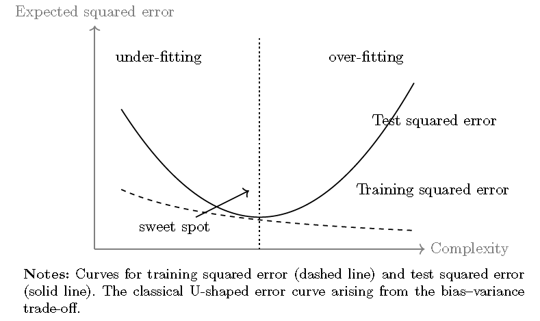
Thus, the ESE is composed of the squared bias, the variance of the prediction (which is a random variable due to data variation \(\mathcal{D}\)), and the irreducible error. The key insight is that increasing model complexity, such as by including more inputs, typically reduces bias but increases variance. This trade-off can lead to overfitting, where models perform well on the training data but poorly on new, unseen data. There is, therefore, an optimal point at which the predictive error is minimized (see the next Figure).70
To avoid overfitting in machine learning, an important step called cross-validation is often employed. This involves splitting the dataset into multiple parts (called folds) and systematically training and testing models on these parts (Hastie, Tibshirani, and Friedman 2009; Bradley Efron and Hastie 2021). The main goal is to evaluate how well models generalize to “unseen data”.
There is a compelling justification for cross-validation within Bayesian inference proposed by J. Bernardo and Smith (1994) in their section 6.1.6. The point of departure is to assume an \(\mathcal{M}-open\) view of nature, in which there exists a set of models \[ \mathcal{M} = \{M_j : j \in J\} \] under comparison, but none of them represents the true data-generating process, which is assumed to be unknown. Nevertheless, we can compare the models in \(\mathcal{M}\) based on their posterior risk functions (see Chapter 1) without requiring the specification of a true model. In this framework, we select the model that minimizes the posterior expected loss. Unfortunately, we cannot explicitly compute this posterior expected loss due to the lack of knowledge of the true posterior distribution under the \(\mathcal{M}-open\) assumption.71
Given the expected loss conditional on model \(j\) for a predictive problem, where the action \(a\) is chosen to minimize the posterior expected loss:
\[ \mathbb{E}_{y_0}[L(Y_0,a) \mid M_j, \mathbf{y}] = \int_{\mathcal{Y}_0} L(y_0, a \mid M_j, \mathbf{y}) \, \pi(y_0 \mid \mathbf{y}) \, dy_0, \]
we note that there are \(N\) possible partitions of the dataset \[ \mathbf{y} = \{y_1, y_2, \dots, y_N\} \] following a leave-one-out strategy, i.e., \[ \mathbf{y} = \{\mathbf{y}_{-k}, y_k\}, \quad k = 1, \dots, N, \] where \(\mathbf{y}_{-k}\) denotes the dataset excluding observation \(y_k\). Assuming that \(\mathbf{y}\) is exchangeable (i.e., its joint distribution is invariant to reordering) and that \(N\) is large, then \(\mathbf{y}_{-k}\) and \(y_k\) are good proxies for \(\mathbf{y}\) and \(y_0\), respectively. Consequently,
\[ \frac{1}{K} \sum_{k=1}^K L(y_k, a \mid M_j, \mathbf{y}_{-k}) \stackrel{p}{\rightarrow} \int_{\mathcal{Y}_0} L(y_0, a \mid M_j, \mathbf{y}) \, \pi(y_0 \mid \mathbf{y}) \, dy_0, \]
by the law of large numbers, as \(N \to \infty\) and \(K \to \infty\).
Thus, we can select a model by minimizing the expected squared error based on its expected predictions \(\mathbb{E}[y_k \mid M_j, \mathbf{y}_{-k}]\); that is, we select the model with the lowest value of
\[ \frac{1}{K} \sum_{k=1}^K \left( \mathbb{E}[y_k \mid M_j, \mathbf{y}_{-k}] - y_k \right)^2. \]
Note that if we want to compare two models based on their relative predictive accuracy using the log-score function (G. M. Martin et al. 2022), we select model \(j\) if
\[ \int_{\mathcal{Y}_0} \log\frac{p(y_0 \mid M_j, \mathbf{y})}{p(y_0 \mid M_l, \mathbf{y})} \, \pi(y_0 \mid \mathbf{y}) \, dy_0 > 0. \]
However, we know that
\[ \frac{1}{K}\sum_{k=1}^K\log\frac{p(y_k \mid M_j, \mathbf{y}_{-k})}{p(y_k \mid M_l, \mathbf{y}_{-k})} \stackrel{p}{\rightarrow} \int_{\mathcal{Y}_0} \log\frac{p(y_0 \mid M_j, \mathbf{y})}{p(y_0 \mid M_l, \mathbf{y})} \, \pi(y_0 \mid \mathbf{y}) \, dy_0, \]
by the law of large numbers as \(N \to \infty\) and \(K \to \infty\).
This implies that we select model \(j\) over model \(l\) if
\[ \prod_{k=1}^K \left( \frac{p(y_k \mid M_j, \mathbf{y}_{-k})}{p(y_k \mid M_l, \mathbf{y}_{-k})} \right)^{1/K} = \prod_{k=1}^K \left( B_{jl}(y_k, \mathbf{y}_{-k}) \right)^{1/K} > 1, \]
where \(B_{jl}(y_k, \mathbf{y}_{-k})\) is the Bayes factor comparing model \(j\) to model \(l\), based on the posterior \(\pi(\boldsymbol{\theta}_m \mid M_m, \mathbf{y}_{-k})\) and the predictive \(\pi(y_k \mid \boldsymbol{\theta}_m)\), for \(m \in \{j, l\}\).
Thus, under the log-score function, cross-validation reduces to the geometric average of Bayes factors that evaluate predictive performance based on the leave-one-out samples \(\mathbf{y}_{-k}\).
References
However, recent developments show that powerful modern machine learning methods, such as deep neural networks, often overfit and yet generalize remarkably well on unseen data. This phenomenon is known as double descent or benign overfitting (Belkin et al. 2019; Bartlett et al. 2020; Hastie et al. 2022).↩︎
This is not the case under an \(\mathcal{M}-closed\) view of nature, where one of the candidate models is assumed to be the true data-generating process. In that setting, the posterior distribution becomes a mixture distribution with mixing probabilities given by the posterior model probabilities (see Chapter 10).↩︎