5.2 Univariate models
After deploying our GUI (see Figure 5.1), the user should select Univariate Models from the top panel. Then, Figure 5.2 is displayed, showing a radio button on the left-hand side that lists the specific models within this category. In particular, users can see that the normal model is selected from the univariate models class.
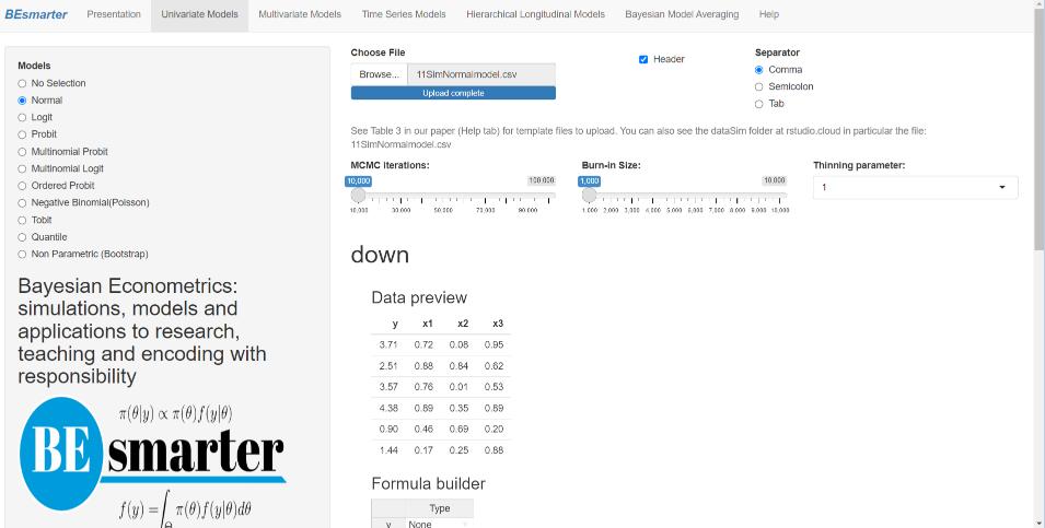
Figure 5.2: Univariate models: Specification.
The right-hand panel then displays a widget for uploading the input dataset, which must be a csv file with headers in the first row. Users must also select the type of separator used in the input file — comma, semicolon, or tab — (see the DataSim and DataApp folders for input file templates). Once the dataset is uploaded, users can preview the data. Range sliders allow users to set the number of iterations for the Markov Chain Monte Carlo algorithm, specify the burn-in period, and adjust the thinning parameter (see the following chapters in this part of the book for technical details).
Next, users must specify the model equation. This can be done using the formula builder, where they select the dependent and independent variables and then click on the Build Formula tab. The equation is displayed in the Main Equation window, formatted according to R syntax, for example, \(y \sim x1 + x2 + x3\). Users can modify this expression as needed to include higher-order terms, interaction effects, or other transformations. These modifications must follow standard formula syntax.29
By default, univariate models include an intercept, except for ordered probit models, where the specification must explicitly exclude it due to identification constraints (see details below).30 Thus, users should specify this explicitly as follows: \(y \sim x1 + x2 + x3 - 1\).
Finally, users must define the prior hyperparameters. For example, in the normal–inverse-gamma model, these include the mean vector, covariance matrix, shape parameter, and scale parameter (see Figure 5.3). However, our GUI uses noninformative hyperparameters by default across all modeling frameworks, so this step is optional.
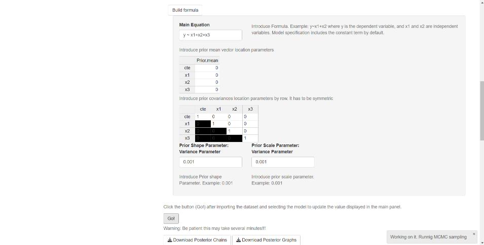
Figure 5.3: Univariate models: Priors.
After completing the specification process, users should click the Go! button to initiate estimation (see Figure 5.3). Once the process is complete, the GUI displays summary statistics and convergence diagnostics. In addition, widgets allow users to download the posterior chains (as csv files) and graphs (as pdf or eps files). Note that in the results — summary tables, posterior chains, and graphs — the coefficients are ordered such that location parameters appear first, followed by scale parameters.
For multinomial models (probit and logit), the dataset must be structured as follows: the first column should contain the dependent variable, followed by alternative-specific regressors (e.g., alternatives’ price), and then non-alternative-specific regressors (e.g., income). The formula builder allows users to specify the dependent variable as well as both types of independent variables (see technical details in the next chapter). Users must also define the base category, the number of alternatives (which is also required for ordered probit models), the number of alternative-specific regressors, and the number of non-alternative-specific regressors (see Figure 5.4).
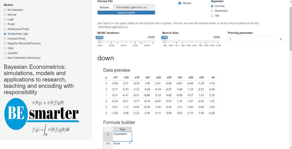
Figure 5.4: Univariate models: Multinomial.
For multinomial logit models, users can additionally specify a tuning parameter corresponding to the degrees of freedom of the Metropolis–Hastings algorithm (see technical details in the next chapter). This tuning option is available in our GUI given that estimation relies on the Metropolis–Hastings algorithm.
In the results of these models, the coefficients are ordered as follows:
- Intercepts (cte\(_l\) in the summary display, where \(l\) represents the alternative).
- Non-alternative-specific regressors (NAS\(_{jl}\) in the summary display, where \(l\) represents the alternative and \(j\) the non-alternative-specific regressor).
- Alternative-specific regressors (AS\(_{j}\) in the summary display, where \(j\) represents the alternative-specific regressor).
Note that the non-alternative-specific regressors associated with the base category are set to zero and do not appear in the results. Additionally, due to identification constraints in multinomial and multivariate probit models, some coefficients in the main diagonal of the covariance matrix remain constant.
For the negative binomial model, users must specify a dispersion parameter (see the next chapter for details). Similarly, for Tobit and quantile models, users need to define the censorship points and quantiles, respectively.
The Bayesian bootstrap method only requires uploading a dataset, specifying the number of MCMC iterations, burn-in size, and defining the equation (see Figure 5.5). The input file should follow the same structure as the one used for the univariate normal model.
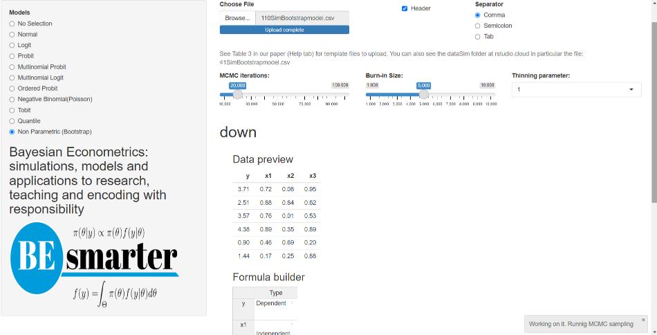
Figure 5.5: Univariate models: Bootstrap.
See https://www.rdocumentation.org/packages/stats/versions/3.6.2/topics/formula↩︎
An identification issue arises when multiple sets of model parameters yield the same likelihood function value.↩︎