12.3 Bayesian additive regression trees
A Classification and Regression Tree (CART) is a method used to predict outcomes based on inputs without assuming a parametric model. It is referred to as a classification tree when the outcome variable is qualitative, and as a regression tree when the outcome variable is quantitative. The method works by recursively partitioning the dataset into smaller, more homogeneous subsets using decision rules based on the input variables. For regression tasks, CART selects splits that minimize prediction error, typically measured by the sum of squared residuals. For classification problems, it aims to create the purest possible groups, using criteria such as Gini impurity or entropy. The result is a tree-like structure in which each internal node represents a decision based on one variable, and each leaf node corresponds to a prediction. CART was popularized in the statistical community by Breiman et al. (1984).
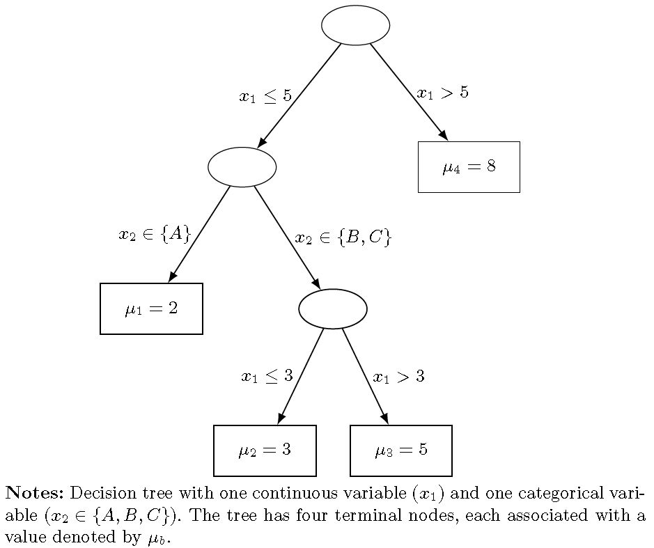
The following figure displays a binary regression tree with two variables: one continuous (\(x_1\)) and one categorical (\(x_2 \in \{A, B, C\}\)). The tree has seven nodes in total, four of which are terminal nodes (\(B = 4\)), dividing the input space \(\mathbf{x} = (x_1, x_2)\) into four non-overlapping regions. Each internal node indicates the splitting variable and rule, while each terminal node shows the value \(\theta_b\), representing the conditional mean of \(y\) given \(\mathbf{x}\).
The first split is based on the rule \(x_1 \leq 5\) (left) versus \(x_1 > 5\) (right). The leftmost terminal node corresponds to \(x_2 \in \{A\}\) with \(\mu_1 = 2\). The second terminal node, with \(\mu_2 = 3\), is defined by \(x_1 \leq 3\) and \(x_2 \in \{B, C\}\). The third node assigns \(\mu_3 = 5\) for \(3 < x_1 \leq 5\) and \(x_2 \in \{B, C\}\). Finally, the rightmost terminal node assigns \(\mu_4 = 8\) for all observations with \(x_1 > 5\).
We can view a CART model as specifying the conditional distribution of \(y\) given the vector of features \(\mathbf{x} = [x_1, x_2, \dots, x_K]^{\top}\). There are two main components: (i) the binary tree structure \(T\), which consists of a sequence of binary decision rules of the form \(x_k \in A\) versus \(x_k \notin A\), where \(A\) is a subset of the range of \(x_k\), and \(B\) terminal nodes that define a non-overlapping and exhaustive partition of the input space; and (ii) the parameter vector \(\boldsymbol{\theta} = [\mu_1, \mu_2, \dots, \mu_B]^{\top}\) and \(\sigma^2\), where each \(\mu_b\) corresponds to the parameter associated with terminal node \(b\), and \(\sigma^2\) is the variance. Consequently, the response \(y \mid \mathbf{x} \sim p(y \mid \mu_b,\sigma^2)\) if \(\mathbf{x}\) belongs to the region associated with terminal node \(b\), where \(p\) denotes a parametric distribution indexed by \(\mu_b\) and \(\sigma^2\).
Assuming that \(y_{bi}\) is independently and identically distributed within each terminal node and independently across nodes, for \(b = 1, 2, \dots, B\) and \(i = 1, 2, \dots, n_b\), we have:
\[ p(\mathbf{y} \mid \mathbf{x}, T, \boldsymbol{\theta}, \sigma^2) = \prod_{b=1}^B p(\mathbf{y}_b \mid \mu_b,\sigma^2) = \prod_{b=1}^B \prod_{i=1}^{n_b} p(y_{bi} \mid \mu_b,\sigma^2), \]
where \(\mathbf{y}_b = [y_{b1}, y_{b2}, \dots, y_{bn_b}]^{\top}\) is the set of observations in terminal node \(b\).
Chipman, George, and McCulloch (1998) introduced a Bayesian formulation of CART models, in which inference is carried out through a combination of prior specification on the binary tree structure \(T\) and the parameters \(\boldsymbol{\theta}, \sigma^2 \mid T\), along with a stochastic search strategy based on a Metropolis-Hastings algorithm. The transition kernels used in the algorithm include operations such as growing, pruning, changing, and swapping tree branches, and candidate trees are evaluated based on their marginal likelihood. This approach enables exploration of a richer set of potential tree models and offers a more flexible and effective alternative to the greedy algorithms commonly used in classical CART.
While CART is a simple yet powerful tool, it is prone to overfitting. To mitigate this, ensemble methods such as boosting, bagging, and random forests are often used. Boosting combines multiple weak trees sequentially, each correcting the errors of its predecessor, to create a strong predictive model (Freund and Schapire 1997). Bagging builds multiple models on bootstrapped datasets and averages their predictions to reduce variance (Breiman 1996), and random forests extend bagging by using decision trees and adding random input selection at each split to increase model diversity (Breiman 2001). Although a single tree might overfit and generalize poorly, aggregating many randomized trees typically yields more accurate and stable predictions.
Chipman, George, and McCulloch (2010) introduced Bayesian Additive Regression Trees (BART). The starting point is the model:
\[ y_i = f(\mathbf{x}_i) + \mu_i, \]
where \(\mu_i \sim N(0, \sigma^2)\).
Thus, the conditional expectation \(\mathbb{E}[y_i \mid \mathbf{x}_i] = f(\mathbf{x}_i)\) is approximated as
\[\begin{equation} \label{eq:BART} f(\mathbf{x}_i) \approx h(\mathbf{x}_i) = \sum_{j=1}^J g_j(\mathbf{x}_i \mid T_j, \boldsymbol{\theta}_j), \end{equation}\]
that is, \(f(\mathbf{x}_i)\) is approximated by the sum of \(J\) regression trees. Each tree is defined by a structure \(T_j\) and a corresponding set of terminal node parameters \(\boldsymbol{\theta}_j\), where \(g_j(\mathbf{x}_i \mid T_j, \boldsymbol{\theta}_j)\) denotes the function that assigns the value \(\mu_{bj} \in \boldsymbol{\theta}_j\) to \(\mathbf{x}_i\) according to the partition defined by \(T_j\).
The main idea is to construct this sum-of-trees model by imposing a prior that regularizes the fit, ensuring that the individual contribution of each tree remains small. Thus, each tree \(g_j\) explains a small and distinct portion of \(f\). This is achieved through Bayesian backfitting MCMC (Hastie and Tibshirani 2000), where successive fits to the residuals are added. In this sense, BART can be viewed as a Bayesian version of boosting.
Chipman, George, and McCulloch (2010) use the following prior structure:
\[\begin{align*} \pi\left(\{(T_1,\boldsymbol{\theta}_1), \dots, (T_J,\boldsymbol{\theta}_J), \sigma^2\}\right) & = \left[\prod_{j=1}^J \pi(T_j,\boldsymbol{\theta}_j)\right]\pi(\sigma)\\ & = \left[\prod_{j=1}^J \pi(\boldsymbol{\theta}_j \mid T_j) \pi(T_j)\right] \pi(\sigma)\\ & = \left[\prod_{j=1}^J \prod_{b=1}^B \pi(\mu_{bj} \mid T_j) \pi(T_j)\right] \pi(\sigma). \end{align*}\]
The prior for the binary tree structure has three components:
(i) the probability that a node at depth \(d = 0, 1, \dots\) is nonterminal, given by \(\alpha(1 + d)^{-\beta}\), where \(\alpha \in (0,1)\) and \(\beta \in [0, \infty)\), the default values are \(\alpha = 0.95\) and \(\beta = 2\); (ii) a uniform prior over the set of available regressors to define the distribution of splitting variable assignments at each interior node; (iii) a uniform prior over the discrete set of available splitting values to define the splitting rule assignment, conditional on the chosen splitting variable.
The prior for the terminal node parameters \(\pi(\mu_{bj} \mid T_j)\) is specified as \(N(0, 0.5 / (k \sqrt{J}))\). The observed values of \(y\) are scaled and shifted to lie within the range \(y_{\text{min}} = -0.5\) to \(y_{\text{max}} = 0.5\), and the default value \(k = 2\) ensures that
\[ P_{\pi(\mu_{bj} \mid T_j)}\left(\mathbb{E}[y \mid \mathbf{x}] \in (-0.5, 0.5)\right) = 0.95. \]
Note that this prior shrinks the effect of individual trees toward zero, ensuring that each tree contributes only a small amount to the overall prediction. Moreover, although the dependent variable is transformed, there is no need to transform the input variables, since the tree-splitting rules are invariant to monotonic transformations of the regressors.
The prior for \(\sigma^2\) is specified as \(\pi(\sigma^2) \sim v\lambda / \chi^2_v\). Chipman, George, and McCulloch (2010) recommend setting \(v = 3\), and choosing \(\lambda\) such that \(P(\sigma < \hat{\sigma}) = q, q = 0.9\), where \(\hat{\sigma}\) is an estimate of the residual standard deviation from a saturated linear model, i.e., a model including all available regressors when \(K < N\), or the standard deviation of \(y\) when \(K \geq N\).
Finally, regarding the number of trees \(J\), the default value is 200. As \(J\) increases from 1, BART’s predictive performance typically improves substantially until it reaches a plateau, after which performance may degrade very slowly. However, if the primary goal is variable selection, using a smaller \(J\) is preferable, as it facilitates identifying the most important regressors by enhancing the internal competition among variables within a limited number of trees.
To sum up, the default hyperparameters are \((\alpha, \beta, k, J, v, q) = (0.95, 2, 2, 200, 3, 0.9)\); however, cross-validation can be used to tune these hyperparameters if desired. BART’s predictive performance appears to be relatively robust to the choice of hyperparameters, provided they are set to sensible values, except in cases where \(K > N\), in which cross-validated tuning tends to yield better performance, albeit at the cost of increased computational time.
Given this specification, we can use a Gibbs sampler that cycles through the \(J\) trees. At each iteration, we sample from the conditional posterior distribution:
\[ \pi(T_j, \boldsymbol{\theta}_j \mid R_j, \sigma) = \pi(T_j \mid R_j, \sigma) \times \pi(\boldsymbol{\theta}_j \mid T_j, R_j, \sigma), \]
where \(R_j = y - \sum_{k \neq j} g_k(\mathbf{x} \mid T_k, \boldsymbol{\theta}_k)\) represents the residuals excluding the contribution of the \(j\)-th tree.
The posterior distribution \(\pi(T_j \mid R_j, \sigma)\) is explored using a Metropolis-Hastings algorithm, where the candidate tree is generated by one of the following moves (Chipman, George, and McCulloch 1998):
(i) growing a terminal node with probability 0.25;
(ii) pruning a pair of terminal nodes with probability 0.25;
(iii) changing a nonterminal splitting rule with probability 0.4; or
(iv) swapping a rule between a parent and child node with probability 0.1.
The posterior distribution of \(\boldsymbol{\theta}_j\) is the product of the posterior distributions \(\pi(\mu_{jb} \mid T_j, R_j, \sigma)\), which are Gaussian. The posterior distribution of \(\sigma\) is inverse-gamma. The posterior draws of \(\mu_{bj}\) are then used to update the residuals \(R_{j+1}\), allowing the sampler to proceed to the next tree in the cycle. The number of iterations in the Gibbs sampler does not need to be very large; for instance, 200 burn-in iterations and 1,000 post-burn-in iterations typically work well.
As we obtain posterior draws from the sum-of-trees model, we can compute point estimates at each \(\mathbf{x}_i\) using the posterior mean, \(\mathbb{E}[y \mid \mathbf{x}_i] = f(\mathbf{x}_i)\). Additionally, pointwise measures of uncertainty can be derived from the quantiles of the posterior draws. We can also identify the most relevant predictors by tracking the relative frequency with which each regressor appears in the sum-of-trees model across iterations. Moreover, we can perform inference on functionals of \(f\), such as the partial dependence functions (Friedman 2001), which quantify the marginal effects of the regressors.
Specifically, if we are interested in the effect of \(\mathbf{x}_s\) on \(y\), while marginalizing over the remaining variables \(\mathbf{x}_c\), such that \(\mathbf{x} = [\mathbf{x}_s^{\top}, \mathbf{x}_c^{\top}]^{\top}\), the partial dependence function is defined as:
\[ f(\mathbf{x}_s) = \frac{1}{N} \sum_{i=1}^N f(\mathbf{x}_s, \mathbf{x}_{ic}), \]
where \(\mathbf{x}_{ic}\) denotes the \(i\)-th observed value of \(\mathbf{x}_c\) in the dataset.
Note that the calculation of the partial dependence function assumes that a subset of the variables is held fixed while averaging over the remainder. This assumption may be questionable when strong dependence exists among input variables, as fixing some variables while varying others may result in unrealistic or implausible combinations. Therefore, caution is warranted when interpreting the results.
Linero (2018) extended BART models to high-dimensional settings for prediction and variable selection, while Hill (2011) and P. R. Hahn, Murray, and Carvalho (2020) applied them to causal inference. The asymptotic properties of BART models have been studied by Ročková and Saha (2019), Ročková and Pas (2020), and Ročková (2020).
Example: Simulation exercise to study BART performance
We use the BART package (Sparapani, Spanbauer, and McCulloch 2021) in the R software environment to perform estimation, prediction, inference, and marginal analysis using Bayesian Additive Regression Trees. In addition to modeling continuous outcomes, this package also supports dichotomous, categorical, and time-to-event outcomes.
We adopt the simulation setting proposed by Friedman (1991), which is also used by Chipman, George, and McCulloch (2010):
\[ y_i = 10\sin(\pi x_{i1}x_{i2}) + 20(x_{i3}-0.5)^2 + 10 x_{i4} + 5 x_{i5} + \mu_i, \]
where \(\mu_i \sim N(0,1)\), for \(i = 1, 2, \dots, 500\).
We set the hyperparameters to \((\alpha, \beta, k, J, v, q) = (0.95, 2, 2, 200, 3, 0.9)\), with a burn-in of 100 iterations, a thinning parameter of 1, and 1,000 post-burn-in MCMC iterations.
We analyze the trace plot of the posterior draws of \(\sigma\) to assess convergence, compare the true values of \(y\) with the posterior mean and 95% predictive intervals for both the training and test sets (using 80% of the data for training and 20% for testing), and visualize the relative importance of the regressors across different values of \(J = 10, 20, 50, 100, 200\).
####### Bayesian Additive Regression Trees #######
rm(list = ls()); set.seed(10101)
library(BART); library(tidyr)
## Loading required package: nlme##
## Attaching package: 'nlme'## The following object is masked from 'package:dplyr':
##
## collapse## Loading required package: survival##
## Attaching package: 'survival'## The following object is masked from 'package:brms':
##
## kidney##
## Attaching package: 'tidyr'## The following objects are masked from 'package:Matrix':
##
## expand, pack, unpacklibrary(ggplot2); library(dplyr)
N <- 500; K <- 10
# Simulate the dataset
MeanFunct <- function(x){
f <- 10*sin(pi*x[,1]*x[,2]) + 20*(x[,3]-.5)^2+10*x[,4]+5*x[,5]
return(f)
}
sig2 <- 1
e <- rnorm(N, 0, sig2^0.5)
X <- matrix(runif(N*K),N,K)
y <- MeanFunct(X[,1:5]) + e
# Train and test
c <- 0.8
Ntrain <- floor(c * N)
Ntest <- N - Ntrain
X.train <- X[1:Ntrain, ]
y.train <- y[1:Ntrain]
X.test <- X[(Ntrain+1):N, ]
y.test <- y[(Ntrain+1):N]
# Hyperparameters
alpha <- 0.95; beta <- 2; k <- 2
v <- 3; q <- 0.9; J <- 200
# MCMC parameters
MCMCiter <- 1000; burnin <- 100; thinning <- 1
# Estimate BART
BARTfit <- wbart(x.train = X.train, y.train = y.train, x.test = X.test, base = alpha,
power = beta, k = k, sigdf = v, sigquant = q, ntree = J,
ndpost = MCMCiter, nskip = burnin, keepevery = thinning)## *****Into main of wbart
## *****Data:
## data:n,p,np: 400, 10, 100
## y1,yn: -4.287055, -6.380098
## x1,x[n*p]: 0.031887, 0.455171
## xp1,xp[np*p]: 0.373776, 0.051661
## *****Number of Trees: 200
## *****Number of Cut Points: 100 ... 100
## *****burn and ndpost: 100, 1000
## *****Prior:beta,alpha,tau,nu,lambda: 2.000000,0.950000,0.481183,3.000000,1.534927
## *****sigma: 2.807107
## *****w (weights): 1.000000 ... 1.000000
## *****Dirichlet:sparse,theta,omega,a,b,rho,augment: 0,0,1,0.5,1,10,0
## *****nkeeptrain,nkeeptest,nkeeptestme,nkeeptreedraws: 1000,1000,1000,1000
## *****printevery: 100
## *****skiptr,skipte,skipteme,skiptreedraws: 1,1,1,1
##
## MCMC
## done 0 (out of 1100)
## done 100 (out of 1100)
## done 200 (out of 1100)
## done 300 (out of 1100)
## done 400 (out of 1100)
## done 500 (out of 1100)
## done 600 (out of 1100)
## done 700 (out of 1100)
## done 800 (out of 1100)
## done 900 (out of 1100)
## done 1000 (out of 1100)
## time: 6s
## check counts
## trcnt,tecnt,temecnt,treedrawscnt: 1000,1000,1000,1000# Trace plot sigma
keep <- seq(burnin + 1, MCMCiter + burnin, thinning)
df_sigma <- data.frame(iteration = 1:length(keep), sigma = BARTfit$sigma[keep])
ggplot(df_sigma, aes(x = iteration, y = sigma)) + geom_line(color = "steelblue") + labs(title = "Trace Plot of Sigma", x = "Iteration", y = expression(sigma)) + theme_minimal()
# Prediction plot training
train_preds <- data.frame( y_true = y.train, mean = apply(BARTfit$yhat.train, 2, mean),
lower = apply(BARTfit$yhat.train, 2, quantile, 0.025), upper = apply(BARTfit$yhat.train, 2, quantile, 0.975)) %>% arrange(y_true) %>% mutate(index = row_number())
ggplot(train_preds, aes(x = index)) + geom_ribbon(aes(ymin = lower, ymax = upper, fill = "95% Interval"), alpha = 0.4, show.legend = TRUE) + geom_line(aes(y = mean, color = "Predicted Mean")) + geom_line(aes(y = y_true, color = "True y")) + scale_color_manual(name = "Line", values = c("Predicted Mean" = "blue", "True y" = "black")) + scale_fill_manual(name = "Interval", values = c("95% Interval" = "lightblue")) + labs(title = "Training Data: Ordered Predictions with 95% Intervals",
x = "Ordered Index", y = "y") + theme_minimal()
# Prediction plot test
test_preds <- data.frame( y_true = y.test, mean = apply(BARTfit$yhat.test, 2, mean), lower = apply(BARTfit$yhat.test, 2, quantile, 0.025), upper = apply(BARTfit$yhat.test, 2, quantile, 0.975)) %>% arrange(y_true) %>% mutate(index = row_number())
ggplot(test_preds, aes(x = index)) + geom_ribbon(aes(ymin = lower, ymax = upper, fill = "95% Interval"), alpha = 0.4, show.legend = TRUE) + geom_line(aes(y = mean, color = "Predicted Mean")) + geom_line(aes(y = y_true, color = "True y")) + scale_color_manual(name = "Line", values = c("Predicted Mean" = "blue", "True y" = "black")) + scale_fill_manual(name = "Interval", values = c("95% Interval" = "lightblue")) + labs(title = "Test Data: Ordered Predictions with 95% Intervals",
x = "Ordered Index", y = "y") + theme_minimal()
# Relevant regressors
Js <- c(10, 20, 50, 100, 200)
VarImportance <- matrix(0, length(Js), K)
l <- 1
for (j in Js){
BARTfit <- wbart(x.train = X.train, y.train = y.train, x.test = X.test, base = alpha,
power = beta, k = k, sigdf = v, sigquant = q, ntree = j,
ndpost = MCMCiter, nskip = burnin, keepevery = thinning)
VarImportance[l, ] <- BARTfit[["varcount.mean"]]/j
l <- l + 1
}## *****Into main of wbart
## *****Data:
## data:n,p,np: 400, 10, 100
## y1,yn: -4.287055, -6.380098
## x1,x[n*p]: 0.031887, 0.455171
## xp1,xp[np*p]: 0.373776, 0.051661
## *****Number of Trees: 10
## *****Number of Cut Points: 100 ... 100
## *****burn and ndpost: 100, 1000
## *****Prior:beta,alpha,tau,nu,lambda: 2.000000,0.950000,2.151914,3.000000,1.534927
## *****sigma: 2.807107
## *****w (weights): 1.000000 ... 1.000000
## *****Dirichlet:sparse,theta,omega,a,b,rho,augment: 0,0,1,0.5,1,10,0
## *****nkeeptrain,nkeeptest,nkeeptestme,nkeeptreedraws: 1000,1000,1000,1000
## *****printevery: 100
## *****skiptr,skipte,skipteme,skiptreedraws: 1,1,1,1
##
## MCMC
## done 0 (out of 1100)
## done 100 (out of 1100)
## done 200 (out of 1100)
## done 300 (out of 1100)
## done 400 (out of 1100)
## done 500 (out of 1100)
## done 600 (out of 1100)
## done 700 (out of 1100)
## done 800 (out of 1100)
## done 900 (out of 1100)
## done 1000 (out of 1100)
## time: 1s
## check counts
## trcnt,tecnt,temecnt,treedrawscnt: 1000,1000,1000,1000
## *****Into main of wbart
## *****Data:
## data:n,p,np: 400, 10, 100
## y1,yn: -4.287055, -6.380098
## x1,x[n*p]: 0.031887, 0.455171
## xp1,xp[np*p]: 0.373776, 0.051661
## *****Number of Trees: 20
## *****Number of Cut Points: 100 ... 100
## *****burn and ndpost: 100, 1000
## *****Prior:beta,alpha,tau,nu,lambda: 2.000000,0.950000,1.521633,3.000000,1.534927
## *****sigma: 2.807107
## *****w (weights): 1.000000 ... 1.000000
## *****Dirichlet:sparse,theta,omega,a,b,rho,augment: 0,0,1,0.5,1,10,0
## *****nkeeptrain,nkeeptest,nkeeptestme,nkeeptreedraws: 1000,1000,1000,1000
## *****printevery: 100
## *****skiptr,skipte,skipteme,skiptreedraws: 1,1,1,1
##
## MCMC
## done 0 (out of 1100)
## done 100 (out of 1100)
## done 200 (out of 1100)
## done 300 (out of 1100)
## done 400 (out of 1100)
## done 500 (out of 1100)
## done 600 (out of 1100)
## done 700 (out of 1100)
## done 800 (out of 1100)
## done 900 (out of 1100)
## done 1000 (out of 1100)
## time: 1s
## check counts
## trcnt,tecnt,temecnt,treedrawscnt: 1000,1000,1000,1000
## *****Into main of wbart
## *****Data:
## data:n,p,np: 400, 10, 100
## y1,yn: -4.287055, -6.380098
## x1,x[n*p]: 0.031887, 0.455171
## xp1,xp[np*p]: 0.373776, 0.051661
## *****Number of Trees: 50
## *****Number of Cut Points: 100 ... 100
## *****burn and ndpost: 100, 1000
## *****Prior:beta,alpha,tau,nu,lambda: 2.000000,0.950000,0.962365,3.000000,1.534927
## *****sigma: 2.807107
## *****w (weights): 1.000000 ... 1.000000
## *****Dirichlet:sparse,theta,omega,a,b,rho,augment: 0,0,1,0.5,1,10,0
## *****nkeeptrain,nkeeptest,nkeeptestme,nkeeptreedraws: 1000,1000,1000,1000
## *****printevery: 100
## *****skiptr,skipte,skipteme,skiptreedraws: 1,1,1,1
##
## MCMC
## done 0 (out of 1100)
## done 100 (out of 1100)
## done 200 (out of 1100)
## done 300 (out of 1100)
## done 400 (out of 1100)
## done 500 (out of 1100)
## done 600 (out of 1100)
## done 700 (out of 1100)
## done 800 (out of 1100)
## done 900 (out of 1100)
## done 1000 (out of 1100)
## time: 1s
## check counts
## trcnt,tecnt,temecnt,treedrawscnt: 1000,1000,1000,1000
## *****Into main of wbart
## *****Data:
## data:n,p,np: 400, 10, 100
## y1,yn: -4.287055, -6.380098
## x1,x[n*p]: 0.031887, 0.455171
## xp1,xp[np*p]: 0.373776, 0.051661
## *****Number of Trees: 100
## *****Number of Cut Points: 100 ... 100
## *****burn and ndpost: 100, 1000
## *****Prior:beta,alpha,tau,nu,lambda: 2.000000,0.950000,0.680495,3.000000,1.534927
## *****sigma: 2.807107
## *****w (weights): 1.000000 ... 1.000000
## *****Dirichlet:sparse,theta,omega,a,b,rho,augment: 0,0,1,0.5,1,10,0
## *****nkeeptrain,nkeeptest,nkeeptestme,nkeeptreedraws: 1000,1000,1000,1000
## *****printevery: 100
## *****skiptr,skipte,skipteme,skiptreedraws: 1,1,1,1
##
## MCMC
## done 0 (out of 1100)
## done 100 (out of 1100)
## done 200 (out of 1100)
## done 300 (out of 1100)
## done 400 (out of 1100)
## done 500 (out of 1100)
## done 600 (out of 1100)
## done 700 (out of 1100)
## done 800 (out of 1100)
## done 900 (out of 1100)
## done 1000 (out of 1100)
## time: 3s
## check counts
## trcnt,tecnt,temecnt,treedrawscnt: 1000,1000,1000,1000
## *****Into main of wbart
## *****Data:
## data:n,p,np: 400, 10, 100
## y1,yn: -4.287055, -6.380098
## x1,x[n*p]: 0.031887, 0.455171
## xp1,xp[np*p]: 0.373776, 0.051661
## *****Number of Trees: 200
## *****Number of Cut Points: 100 ... 100
## *****burn and ndpost: 100, 1000
## *****Prior:beta,alpha,tau,nu,lambda: 2.000000,0.950000,0.481183,3.000000,1.534927
## *****sigma: 2.807107
## *****w (weights): 1.000000 ... 1.000000
## *****Dirichlet:sparse,theta,omega,a,b,rho,augment: 0,0,1,0.5,1,10,0
## *****nkeeptrain,nkeeptest,nkeeptestme,nkeeptreedraws: 1000,1000,1000,1000
## *****printevery: 100
## *****skiptr,skipte,skipteme,skiptreedraws: 1,1,1,1
##
## MCMC
## done 0 (out of 1100)
## done 100 (out of 1100)
## done 200 (out of 1100)
## done 300 (out of 1100)
## done 400 (out of 1100)
## done 500 (out of 1100)
## done 600 (out of 1100)
## done 700 (out of 1100)
## done 800 (out of 1100)
## done 900 (out of 1100)
## done 1000 (out of 1100)
## time: 6s
## check counts
## trcnt,tecnt,temecnt,treedrawscnt: 1000,1000,1000,1000rownames(VarImportance) <- c("10", "20", "50", "100", "200")
colnames(VarImportance) <- as.character(1:10)
importance_df <- as.data.frame(VarImportance) %>% mutate(trees = rownames(.)) %>%
pivot_longer(cols = -trees, names_to = "variable", values_to = "percent_used")
importance_df$variable <- as.numeric(importance_df$variable)
importance_df$trees <- factor(importance_df$trees, levels = c("10", "20", "50", "100", "200"))
ggplot(importance_df, aes(x = variable, y = percent_used, color = trees, linetype = trees)) + geom_line() + geom_point() + scale_color_manual(values = c("10" = "red", "20" = "green", "50" = "blue", "100" = "cyan", "200" = "magenta")) + scale_x_continuous(breaks = 1:10) + labs(x = "variable", y = "percent used", color = "#trees", linetype = "#trees") + theme_minimal()
The first figure displays the trace plot of \(\sigma\), which appears to have reached a stationary distribution. However, the posterior draws are slightly lower than the true value (1).
The second and third figures compare the true values of \(y\) with the posterior mean and 95% predictive intervals. The BART model performs well in both sets, and the intervals in the test set are notably wider than those in the training set.
The last figure shows the relative frequency with which each variable is used in the trees, a measure of variable relevance. When the number of trees is small, the algorithm more clearly identifies the most relevant predictors (variables 1–5). As the number of trees increases, this discrimination gradually disappears.