13.3 Conditional independence assumption (CIA)
In practice, researchers often work with observational data, where the treatment status is not randomly assigned because units actively choose the treatment they receive. In an RCT, the assignment mechanism is determined by chance, whereas in observational studies it is driven by choice. In these situations, we can identify the causal effect if the conditional independence assumption (CIA) holds. This assumption states that the potential outcomes are independent of the treatment status, conditional on a set of observed pre-treatment variables: \[ \{ Y_i(1), Y_i(0) \} \perp D_i \mid \mathbf{X}_i. \]
This means that, conditional on the pre-treatment variables \(\mathbf{X}_i\), treatment assignment is as good as random. This property is known as unconfoundedness given \(\mathbf{X}_i\), or equivalently, the no unmeasured confounders assumption. When this condition is combined with the requirement that, for all possible values of \(\mathbf{X}_i\), there is a positive probability of receiving each treatment level (\(0 < P(D_i = 1 \mid \mathbf{X}_i) < 1\)), the joint condition is referred to as strong ignorability. Identification of average causal effects in this setting also requires the SUTVA.
Note that under the CIA, \[\begin{align} \text{ATE} &= \mathbb{E}[Y_i(1)] - \mathbb{E}[Y_i(0)] \\ &= \mathbb{E}_{\mathbf{X}}\left\{ \mathbb{E}[Y_i(1)\mid \mathbf{X}_i] - \mathbb{E}[Y_i(0)\mid \mathbf{X}_i] \right\} \\ &= \mathbb{E}_{\mathbf{X}}\left\{ \mathbb{E}[Y_i(1)\mid \mathbf{X}_i, D_i=1] - \mathbb{E}[Y_i(0)\mid \mathbf{X}_i, D_i=0] \right\} \\ &= \mathbb{E}_{\mathbf{X}}\left\{ \mathbb{E}[Y_i\mid \mathbf{X}_i, D_i=1] - \mathbb{E}[Y_i\mid \mathbf{X}_i, D_i=0] \right\} \\ &= \mathbb{E}_{\mathbf{X}}\left\{ \tau(\mathbf{X}_i) \right\}, \tag{13.1} \end{align}\]
where the second equality follows from the law of iterated expectations, the third uses CIA, and \[ \tau(\mathbf{X}_i) = \mathbb{E}[Y_i \mid \mathbf{X}_i, D_i=1] - \mathbb{E}[Y_i \mid \mathbf{X}_i, D_i=0] \] is the conditional average treatment effect (CATE) at covariate value \(\mathbf{X}_i\), which captures treatment effect heterogeneity across different values of \(\mathbf{X}\). Therefore, the ATE is the expectation of the CATE over the distribution of \(\mathbf{X}\).
The foolowing figure illustrates the causal structure underlying the CIA. We follow the convention that time flows from left to right. Here, \(\mathbf{X}\) —a vector of pre-treatment variables or confounders— influences both the treatment (\(D\)) and the outcome (\(Y\)). Under the CIA, we can identify the causal effect of \(D\) on \(Y\) by adjusting for \(\mathbf{X}\) because this causal structure satisfies the back-door criterion. This criterion states that a set of variables \(\mathbf{X}\) satisfies the condition for identifying the effect of \(D\) on \(Y\) if no variable in \(\mathbf{X}\) is a descendant of \(D\) and \(\mathbf{X}\) blocks every back-door path from \(D\) to \(Y\). A back-door path is any path from \(D\) to \(Y\) that begins with an arrow pointing into \(D\).
In Exercise 3, we ask to construct the DAG of the following figure, verify that it is acyclic, and check whether the causal effect of \(D\) on \(Y\) is identifiable by controlling for \(\mathbf{X}\) using the package dagitty.
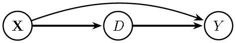
Figure 13.3: Directed Acyclic Graph (DAG) implied by the Conditional Independence Assumption (CIA).
This figure displays the SWIG.
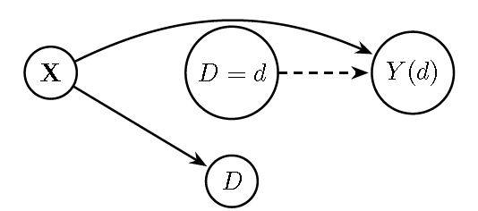
Figure 13.4: Single-World Intervention Graph (SWIG) for \(do(D=d)\): The treatment \(D\) is split into the fixed intervention \(D=d\) and its natural value. The outcome is replaced by \(Y(d)\). \(X\) still influences \(Y(d)\), so adjustment for \(X\) is needed for identification.
The simple regression framework of the previous section can be extended to a multiple linear regression model by including the pre-treatment variables; therefore, if the CEF is linear in the treatment and pre-treatment variables: \[ Y_i = \beta_0 + \tau D_i + \mathbf{X}_i^{\top}\boldsymbol{\beta} + \mu_i. \]
Note that, by assumption in RCTs, \(D_i\) and \(\mathbf{X}_i\) are independent. Thus, the identification of \(\tau\) is not affected under random assignment; however, including \(\mathbf{X}_i\) helps explain part of the variability in \(Y_i\), thereby improving the precision of the estimates.
On the other hand, if the CIA is satisfied, the error term in the linear regression is defined as \[ \mu_i = Y_i(0) - \mathbb{E}[Y_i(0) \mid \mathbf{X}_i]. \]
Thus, \[ \mathbb{E}[\mu_i \mid D_i, \mathbf{X}_i] = \mathbb{E}[Y_i(0) - \mathbb{E}[Y_i(0) \mid \mathbf{X}_i] \mid D_i, \mathbf{X}_i] = \mathbb{E}[Y_i(0) \mid D_i, \mathbf{X}_i] - \mathbb{E}[Y_i(0) \mid \mathbf{X}_i]. \]
By the CIA, \(Y_i(0) \perp D_i \mid \mathbf{X}_i\), so: \[ \mathbb{E}[Y_i(0) \mid D_i, \mathbf{X}_i] = \mathbb{E}[Y_i(0) \mid \mathbf{X}_i]. \]
Therefore: \[\begin{equation*} \mathbb{E}[\mu_i \mid D_i, \mathbf{X}_i] = 0 \end{equation*}\]
This condition is known as conditional mean independence: after controlling for \(\mathbf{X}_i\), treatment assignment is independent of unobserved determinants of the outcome. It justifies unbiased estimation of \(\tau\) by regression adjustment in observational studies.
Example: Treatment effect of 401(k) eligibility on net financial assets
We study the average treatment effect of eligibility (e401) for participation in the 401(k) retirement savings plan in the United States on net financial assets (net_tfa) using the dataset 401k.csv. The rationale for the exogeneity of 401(k) eligibility is that it becomes exogenous after conditioning on observable characteristics related to job choice, which may correlate with whether a firm offers this retirement plan (Victor Chernozhukov et al. 2024).
Accordingly, we control for the following covariates: age (age), income (inc), family size (fsize), years of education (educ), a marital status indicator (marr), a two-earner status indicator (twoearn), a defined benefit pension status indicator (db), an IRA participation indicator (pira), and a home ownership indicator (hown). Under this specification, the key assumption is that eligibility is conditionally independent of net financial assets given these covariates (Victor Chernozhukov et al. 2024).
We can use the framework in Section 6.1 to estimate the average treatment effect of 401(k) eligibility on net financial assets. The following code shows how to obtain the posterior distribution of this effect. The figure displays the posterior distribution of the treatment effect: the 95% credible interval is (USD 3,473, USD 8,371), and the posterior mean is USD 5,903.
# 401k: Treatment effects
rm(list = ls())
set.seed(10101)

library(MCMCpack)
library(coda)
library(ggplot2)

mydata <- read.csv("https://raw.githubusercontent.com/BEsmarter-consultancy/BSTApp/refs/heads/master/DataApp/401k.csv", sep = ",", header = TRUE, quote = "")
attach(mydata )
## The following object is masked from DataIntRate (pos = 28):
##
## i3## The following object is masked from DataIntRate (pos = 30):
##
## i3y <- net_tfa
# net_tfa: net financial assets
# Regressors quantity including intercept
X <- cbind(e401, age, inc, fsize, educ, marr, twoearn, db, pira, hown, 1)
# e401: 401k eligibility
# age, income, family size, years of education, marital status indicator, two-earner status indicator, defined benefit pension status indicator, IRA participation indicator, and home ownership indicator.
# Posterior distributions using packages: MCMCpack sets the model in terms of the precision matrix. We use default parameters
posterior <- MCMCpack::MCMCregress(y~X-1)
summary(coda::mcmc(posterior))##
## Iterations = 1:10000
## Thinning interval = 1
## Number of chains = 1
## Sample size per chain = 10000
##
## 1. Empirical mean and standard deviation for each variable,
## plus standard error of the mean:
##
## Mean SD Naive SE Time-series SE
## Xe401 5.903e+03 1.265e+03 1.265e+01 1.265e+01
## Xage 6.248e+02 6.020e+01 6.020e-01 6.020e-01
## Xinc 9.356e-01 3.028e-02 3.028e-04 3.028e-04
## Xfsize -1.019e+03 4.492e+02 4.492e+00 4.492e+00
## Xeduc -6.425e+02 2.257e+02 2.257e+00 2.257e+00
## Xmarr 7.390e+02 1.802e+03 1.802e+01 1.773e+01
## Xtwoearn -1.922e+04 1.580e+03 1.580e+01 1.580e+01
## Xdb -4.916e+03 1.371e+03 1.371e+01 1.371e+01
## Xpira 2.953e+04 1.449e+03 1.449e+01 1.449e+01
## Xhown 1.188e+03 1.320e+03 1.320e+01 1.284e+01
## X -3.290e+04 4.247e+03 4.247e+01 4.247e+01
## sigma2 3.106e+09 4.360e+07 4.360e+05 4.177e+05
##
## 2. Quantiles for each variable:
##
## 2.5% 25% 50% 75% 97.5%
## Xe401 3.473e+03 5.044e+03 5.898e+03 6.759e+03 8.371e+03
## Xage 5.070e+02 5.844e+02 6.248e+02 6.647e+02 7.443e+02
## Xinc 8.765e-01 9.150e-01 9.358e-01 9.554e-01 9.947e-01
## Xfsize -1.886e+03 -1.329e+03 -1.024e+03 -7.142e+02 -1.269e+02
## Xeduc -1.076e+03 -7.957e+02 -6.461e+02 -4.916e+02 -1.883e+02
## Xmarr -2.794e+03 -4.825e+02 7.436e+02 1.951e+03 4.268e+03
## Xtwoearn -2.235e+04 -2.029e+04 -1.923e+04 -1.815e+04 -1.616e+04
## Xdb -7.611e+03 -5.851e+03 -4.919e+03 -4.004e+03 -2.189e+03
## Xpira 2.672e+04 2.855e+04 2.952e+04 3.051e+04 3.242e+04
## Xhown -1.396e+03 3.076e+02 1.181e+03 2.081e+03 3.752e+03
## X -4.125e+04 -3.579e+04 -3.286e+04 -2.999e+04 -2.472e+04
## sigma2 3.021e+09 3.076e+09 3.105e+09 3.135e+09 3.193e+09# Extract posterior samples for e401 (first coefficient)
beta_e401 <- posterior[, 1]
# Convert to data frame for ggplot
df_posterior <- data.frame(beta_e401)
# Plot with ggplot
ggplot(df_posterior, aes(x = beta_e401)) +
geom_density(fill = "steelblue", alpha = 0.6) +
geom_vline(xintercept = mean(beta_e401), color = "red", linetype = "dashed") +
labs(
title = "Posterior Distribution of Treatment Effect (e401)",
x = expression(beta[e401]),
y = "Density"
) +
theme_minimal(base_size = 14)## Don't know how to automatically pick scale for object of type <mcmc>.
## Defaulting to continuous.
Observe that the identification strategy relies on conditioning on \(\mathbf{X}\). However, adding more controls is not always safe because some variables, known as bad controls, can introduce bias if included in the adjustment set (Angrist and Pischke 2009). One important type of bad control is a collider, a variable that is caused by (or is a common effect of) two or more other variables in a DAG. Colliders play a critical role because conditioning on them can create spurious associations between their causes, leading to what is known as collider bias (or selection bias).
The following figure illustrates this situation. Here, \(C\) is a common effect of \(D\) and \(\mathbf{X}\). Conditioning on \(C\) opens an additional path between \(D\) and \(Y\), creating a spurious association that violates the back-door criterion. In particular, the variable \(C\) is a collider on the path \(D \to C \leftarrow \mathbf{X}\). By default, a collider blocks the flow of association along the path on which it lies, so this path is closed when \(C\) is not conditioned on. However, conditioning on \(C\) (or on any descendant of \(C\)) opens this path, creating a spurious association between \(D\) and \(\mathbf{X}\). Since \(\mathbf{X}\) also affects \(Y\), this induces bias in estimating the causal effect of \(D\) on \(Y\).
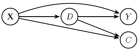
Figure 13.5: Directed Acyclic Graph (DAG): The additional collider \(C\) caused by both \(D\) and \(X\) would open a path between \(D\) and \(X\), inducing bias.
Example: Birth-weight “paradox”, collider bias
The collider bias illustrated in the following DAG, based on Victor Chernozhukov et al. (2024), reflects the well-known Birth-weight “paradox”. This phenomenon arises when conditioning on an intermediate variable (birth weight, \(B\)) induces a spurious association between the binary indicator of smoking (\(S\)) and infant mortality (\(Y\)). In this setting, \(U\) represents unobserved factors that affect both birth weight and infant mortality. Conditioning on \(B\) creates collider bias because it opens a back-door path through the unobserved factors \(U\) (dashed).

Figure 13.6: DAG illustrating the birth-weight paradox: \(S\) (smoking), \(B\) (birth weight), \(Y\) (infant mortality), and \(U\) (other unobserved health factors).
The following code illustrates the bias by performing 100 replications, and the figure shows the distribution of posterior means across these replications. In this setting, the total effect of smoking on infant mortality is 2, consisting of a direct effect of 1 and an indirect effect through birth weight, also equal to 1.
rm(list = ls()); set.seed(10101)
library(MCMCpack); library(dplyr); library(ggplot2)
# Parameters
n <- 1000; true_effect <- 2; replications <- 100
# Store results
results <- data.frame(rep = 1:replications, correct = numeric(replications), biased = numeric(replications))

for (r in 1:replications) {
    # Simulate data under DAG: S -> B -> Y, S -> Y, U -> B, U -> Y
    U <- rnorm(n, 0, 1); S <- rbinom(n, prob = 0.7, size = 1)
    B <- S + U + rnorm(n)
    Y <- S + B + 1.5*U + rnorm(n)
    # Correct model: does NOT condition on collider B
    model_correct <- MCMCregress(Y ~ S, burnin = 1000, mcmc = 3000, verbose = FALSE)
    # Biased model: conditions on collider B
    model_biased <- MCMCregress(Y ~ S + B, burnin = 1000, mcmc = 3000, verbose = FALSE)
    # Posterior means for S
    results$correct[r] <- mean(as.matrix(model_correct)[, "S"])
    results$biased[r] <- mean(as.matrix(model_biased)[, "S"])
}
# Compute bias
results <- results %>% mutate(
bias_correct = correct - true_effect,
bias_biased = biased - true_effect
)
# Average bias and SD
avg_bias <- results %>%
summarise(
mean_correct = mean(bias_correct),
mean_biased = mean(bias_biased),
sd_correct = sd(bias_correct),
sd_biased = sd(bias_biased)
)
print(avg_bias)
## mean_correct mean_biased sd_correct sd_biased
## 1 -0.004798032 -1.755074 0.2161217 0.0948221# Visualization: distribution of posterior means across 100 simulations
df_long <- results %>% dplyr::select(rep, correct, biased) %>% tidyr::pivot_longer(cols = c(correct, biased), names_to = "model", values_to = "estimate")
ggplot(df_long, aes(x = estimate, fill = model)) + geom_density(alpha = 0.5) + geom_vline(xintercept = true_effect, color = "black", linetype = "dashed", linewidth = 1) + labs(title = "Posterior Means Across 100 Simulations", x = expression(paste("Posterior Mean of ", beta[S])), y = "Density") + theme_minimal(base_size = 14)
Collider (selection) bias is one possible source of bias in the identification of causal effects. The well-known Heckman’s sample selection problem in econometrics (Heckman 1979) can be interpreted as a form of collider bias because restricting the analysis to selected observations (e.g., those with positive wages) conditions on a variable that is a common effect of observed and unobserved factors, thereby opening a non-causal path and creating bias. In other words, the sample is no longer representative of the population, which undermines the identification of the causal effect.
Other well-known sources of bias in econometrics include the omission of common causes affecting both the treatment and the outcome, that is, omission of correlated relevant regressors, measurement error in regressors leading to attenuation bias (where the estimated causal effect is biased toward zero), and simultaneous causality, which often arises in systems of equations (see Jeffrey M. Wooldridge (2010) for details). We will discuss these additional sources of bias later.