13.5 Difference-in-differences design (DiD)
In this section, we present how to perform inference and discuss the identification conditions when working with panel (longitudinal) data or repeated cross-sectional data in the difference-in-differences (DiD) framework. In DiD designs, we estimate causal effects by comparing changes over time between groups that receive the treatment and groups that do not (the “control” group). This approach is among the most widely used designs for identifying causal effects (A. Baker et al. 2025). Its origins can be traced back to John Snow, the father of modern epidemiology, who in 1855 analyzed the spread of cholera through water in London (Victor Chernozhukov et al. 2024).
In what follows, we first present the basic two-group, two-period (\(2\times2\)) DiD setup, and then introduce the staggered DiD design.
13.5.1 Classic DiD: two-group and two-period (\(2\times2\)) setup
Following Roth et al. (2023), we consider a setting with two time periods, \(t = 1, 2\), and two groups: a treated group (\(D_i = 1\)) that receives the treatment between periods \(t = 1\) and \(t = 2\), and a control group that never receives the treatment (\(D_i = 0\)). We observe outcomes \(Y_{it}\) and treatment status \(D_i\) for units \(i = 1, 2, \dots, N\), assuming a balanced panel data structure.
Let \(Y_{it}(1)\) denote the potential outcome for unit \(i\) in period \(t\) if it is untreated in the first period and treated in the second, while \(Y_{it}(0)\) denotes the potential outcome if it is never treated. In the DiD framework, the primary estimand of interest is the average treatment effect on the treated (ATT),
\[ \tau_{2} = \mathbb{E}[Y_{i2}(1) - Y_{i2}(0) \mid D_i = 1]. \]
Note that we do not observe \(Y_{i2}(0) \mid D_i = 1\); that is, the outcome in the second period for treated units if they had not received the treatment. Thus, the identification conditions in DiD are designed to express this counterfactual outcome as a function of the data.
There are two key identification assumptions:
1. Parallel trends:
\[ \mathbb{E}[Y_{i2}(0) - Y_{i1}(0) \mid D_i = 1] = \mathbb{E}[Y_{i2}(0) - Y_{i1}(0) \mid D_i = 0], \]
which states that, in the absence of treatment, the average change in outcomes for the treated and control groups would have evolved similarly over time.
2. No anticipation effects:
\[ \mathbb{E}[Y_{i1}(0)\mid D_i=1] = \mathbb{E}[Y_{i1}(1)\mid D_i=1], \]
meaning that the treatment has no causal effect prior to its implementation.
Thus, we can use the parallel trends assumption to express \(\mathbb{E}[Y_{i2}(0) \mid D_i = 1]\) as
\[ \begin{aligned} \mathbb{E}[Y_{i2}(0)\mid D_i = 1] &= \mathbb{E}[Y_{i1}(0) \mid D_i = 1] + \mathbb{E}[Y_{i2}(0) - Y_{i1}(0) \mid D_i = 0] \\ &= \mathbb{E}[Y_{i1}(1) \mid D_i = 1] + \mathbb{E}[Y_{i2}(0) - Y_{i1}(0) \mid D_i = 0] \\ &= \mathbb{E}[Y_{i1} \mid D_i = 1] + \mathbb{E}[Y_{i2} - Y_{i1} \mid D_i = 0], \end{aligned} \]
where the second equality follows from the no anticipation effects assumption.
Therefore,
\[\begin{equation} \tau_2 = \mathbb{E}[Y_{i2} - Y_{i1} \mid D_i = 1] - \mathbb{E}[Y_{i2} - Y_{i1} \mid D_i = 0], \tag{13.2} \end{equation}\]
that is, the ATT is the difference in outcome differences between treated and control units.
The following figure shows a graphical representation of the identification assumptions in DiD (Victor Chernozhukov et al. 2024). Normington et al. (2022) show a DAG representation of DiD.
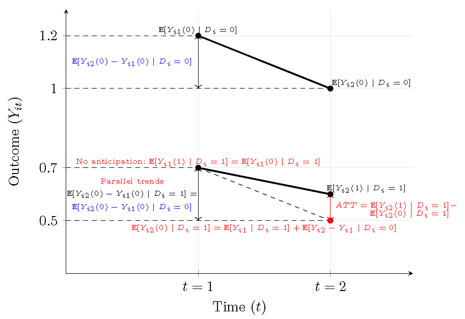
Figure 13.8: Difference-in-Differences: Identification strategy.
Note that we can express the observed outcome in terms of potential outcomes as
\[ Y_{it} = Y_{it}(0) + \big[\,Y_{it}(1) - Y_{it}(0)\,\big] D_i. \]
Therefore,
\[ Y_{i1} = Y_{i1}(0) + \big[\,Y_{i1}(1) - Y_{i1}(0)\,\big] D_i, \]
and
\[ Y_{i2} = Y_{i2}(0) + \big[\,Y_{i2}(1) - Y_{i2}(0)\,\big] D_i. \]
Subtracting the first equation from the second yields
\[ Y_{i2} - Y_{i1} = \underbrace{Y_{i2}(0) - Y_{i1}(0)}_{\text{common trend}} + \underbrace{\big[(Y_{i2}(1) - Y_{i1}(1)) - (Y_{i2}(0) - Y_{i1}(0))\,\big]}_{\text{treatment effect in changes}} D_i. \]
Under the parallel trends assumption, the expected value of the common trend is the same for treated and control units. This assumption is compatible with the linear CEF function
\[ Y_{it} = \alpha_i + \phi_t + \tau_2 D_i + \mu_{it}, \]
which implies
\[ Y_{i2} - Y_{i1} = (\phi_2 - \phi_1) + \tau_2 D_i + (\mu_{i2} - \mu_{i1}). \]
Comparing this expression with the one derived from the potential outcomes framework, it follows that regressing the time difference \(Y_{i2} - Y_{i1}\) on a constant and the treatment indicator \(D_i\) identifies \(\tau_2\), the ATT.
Another common formulation in the linear regression setting that recovers the ATT is the two-way fixed effects (TWFE) model
\[ Y_{it} = \alpha + \alpha_i + \phi_t + \tau_2 \,\big[ D_i \cdot \mathbf{1}(t = 2) \big] + \epsilon_{it}, \]
where \(\mathbf{1}(t = 2)\) is an indicator for the post-treatment period (Roth et al. 2023). The advantage of the regression setting is that it allows for the straightforward calculation of the standard error of the ATT, enabling the construction of confidence or credible intervals under the Frequentist and Bayesian approaches, respectively.
The DiD framework can be extended to condition on covariates. In this case, we assume that the underlying identification assumptions are more plausible among units that are similar in terms of observed characteristics. Thus, the identification assumptions are stated conditional on the exogenous variables.
Therefore, we can use covariates to assess the balance between control and treated groups in terms of levels (\(X\)) or differences (\(\Delta X\)) before and after treatment:
\[ \frac{\bar{X}_1-\bar{X}_2}{\sqrt{\hat{\sigma}_1^2+\hat{\sigma}_2^2}}, \]
where \(\hat{\sigma}_l^2\) is the sample variance of \(X_l\), \(l=\{1,2\}\).
As a rule of thumb, absolute standardized differences greater than 0.25 indicate potentially problematic imbalance (A. Baker et al. 2025). Imbalance in covariates can lead to violations of the parallel trends assumption if these covariates would generate different outcomes under the counterfactual scenarios.
In this setting, the conditional parallel trends assumption becomes
\[\begin{equation} \mathbb{E}[Y_{i2}(0) - Y_{i1}(0) \mid D_i = 1, \mathbf{X}_i] = \mathbb{E}[Y_{i2}(0) - Y_{i1}(0) \mid D_i = 0, \mathbf{X}_i], \ \text{almost surely,} \end{equation}\]
and the no anticipation assumption becomes
\[\begin{equation} \mathbb{E}[Y_{i1}(0) \mid D_i = 1, \mathbf{X}_i] = \mathbb{E}[Y_{i1}(1) \mid D_i = 1, \mathbf{X}_i]. \end{equation}\]
In addition, the overlap assumption is required: there exists a treatment group whose characteristics overlap with those of the control group,
\[ P(D_i = 1 \mid \mathbf{X}_i) < 1 - \epsilon, \ \epsilon >0, \ \text{almost surely, and,} \ P(D_i=1)>0. \]
Following similar arguments as before, we obtain the conditional average treatment effect on the treated (CATT) (A. Baker et al. 2025):
\[ \tau_2(\mathbf{X}_i)= \mathbb{E}[Y_{i2} - Y_{i1} \mid D_i = 1, \mathbf{X}_i] - \mathbb{E}[Y_{i2} - Y_{i1} \mid D_i = 0, \mathbf{X}_i]. \]
The overall ATT can then be recovered by averaging over the distribution of \(\mathbf{X}_i\) in the treated population:
\[ \begin{aligned} \tau_2 & = \mathbb{E}_{\mathbf{X}}\left\{\mathbb{E}[Y_{i2} - Y_{i1} \mid D_i = 1, \mathbf{X}_i] - \mathbb{E}[Y_{i2} - Y_{i1} \mid D_i = 0, \mathbf{X}_i] \mid D_i = 1\right\}\\ &=\mathbb{E}[Y_{i2} - Y_{i1} \mid D_i = 1]-\mathbb{E}_{\mathbf{X}}\left\{\mathbb{E}[Y_{i2} - Y_{i1} \mid D_i = 0, \mathbf{X}_i]\mid D_i=1\right\}, \end{aligned} \]
where the second line uses the law of iterated expectations:
\[ \mathbb{E}_{\mathbf{X}\mid D=1}\!\left( \mathbb{E}[Y_{i2}-Y_{i1} \mid D=1, \mathbf{X}_i] \right) = \mathbb{E}[Y_{i2}-Y_{i1} \mid D=1]. \]
Assuming a linear CEF and a homogeneous ATT, that is, treatment effects do not vary across \(\mathbf{X}_{it}\), we can use the first–difference specification,
\[ \Delta Y_{i2} = \alpha + \beta D_i + \sum_{k=1}^K \beta_k \Delta X_{ik2} + \Delta\mu_{i2}, \]
where \(\Delta Y_{i2} = Y_{i2} - Y_{i1}\) and \(\Delta X_{ik2} = X_{ik2} - X_{ik1}\). This specification identifies the ATT under the homogeneity assumption, in which case \(\tau_2 = \beta\); otherwise, it identifies a weighted average of the conditional ATTs across covariates, with the possibility of negative weights that do not sum to one (non-convex weights) (A. Baker et al. 2025).
An alternative specification is the TWFE
\[ \begin{aligned} Y_{it} & = \alpha + \alpha_i + \phi_t + \beta (\mathbf{1}(t=2)\cdot D_i) + \sum_{k=1}^K \beta_k (\mathbf{1}(t=2)\cdot X_{ik1})\\ & + \sum_{k=1}^K \delta_k (\mathbf{1}(t=2)\cdot D_i \cdot X_{ik1}) + \epsilon_{it}. \end{aligned} \]
This specification can identify heterogeneous ATT under the assumption of a linear CEF.
However, alternative semiparametric and nonparametric approaches, such as outcome regression adjustment, inverse probability weighting, and doubly robust estimators (which combine the first two), are often preferable because they yield consistent estimates under conditional parallel trends without requiring a linear conditional expectation function (CEF) (Abadie 2005; Roth et al. 2023). These approaches typically involve two stages: first, estimating either the conditional mean of the outcome or the propensity score (probability of treatment (Rosenbaum and Rubin 1983)), and second, using these estimates in a plug-in step to perform inference on the ATT. For Bayesian doubly robust frameworks for average treatment effects, see Saarela, Belzile, and Stephens (2016), Yiu, Goudie, and Tom (2020), Luo, Graham, and McCoy (2023), Breunig, Liu, and Yu (2025).
A point to be aware of when performing DiD identification strategies is that the parallel trends assumption is generally not robust to functional form transformations of the outcome. That is, it may hold when the outcome is measured in levels but fail when it is expressed in logarithms. This is because two groups can have the same absolute increase (parallel trends in levels) but different percentage increases (non-parallel in logs).
Note that the parallel trends and no anticipation assumptions in DiD are not fundamentally testable, since they are identifying restrictions about counterfactual outcomes that are never observed. However, we can examine pre-treatment dynamics to assess their plausibility. For instance, we can check for pre-existing differences in trends (“pre-trends”) as a diagnostic for the parallel trends assumption.
Given a pre-treatment period \(t=0\), the no anticipation assumption implies that
\[ \mathbb{E}[Y_{it}(0)] = \mathbb{E}[Y_{it}] \quad \text{for all } i \text{ and } t \leq 0. \]
Thus, one can test whether
\[\begin{equation} \mathbb{E}[Y_{i1}(0) - Y_{i0}(0) \mid D_i = 1] = \mathbb{E}[Y_{i1}(0) - Y_{i0}(0) \mid D_i = 0], \end{equation}\]
which corresponds to checking for differences in pre-treatment trends between treated and control groups.
The results of such tests should be interpreted with caution. Even if pre-trends are perfectly parallel, this does not guarantee that the parallel trends assumption will hold in the post-treatment period. Moreover, there may be power issues: a true pre-existing difference in trends may go undetected if pre-treatment estimates are imprecise due to high variability.
In addition, one can conduct placebo tests by pretending that the policy started earlier and checking whether a spurious effect is detected prior to the true start. This provides indirect evidence on the plausibility of the no anticipation assumption.
Therefore, it is advisable to complement pre-trend diagnostics with sensitivity analyses, incorporating context-specific knowledge about plausible confounding factors.
13.5.2 Staggered (SDiD): G-group and T-period (\(G\times T\)) setup
Many empirical settings are more complex than the two-period, two-group (\(2\times 2\)) design. Nevertheless, even in such settings we can view the design as an aggregation of \(2\times 2\) comparisons between units that receive treatment and units that are not yet treated at the relevant time (A. Baker et al. 2025).
In a setting with multiple periods and different groups, assuming that treatment is an absorbing state —that is, once treated, units remain treated— staggered DiD (SDiD) analyses seek to estimate a weighted average of heterogeneous ATTs, where the weights may be based on economic/policy relevance.
Given \(t = 1, 2, \dots, T\), a unit can be treated at \(t = g > 1\),
\[ Y_{it}(g) := Y_{it}\big(\underbrace{0, \dots, 0}_{g-1}, \underbrace{1, \dots, 1}_{T-g+1}\big) \]
denotes the potential outcome path for a unit treated at \(g\), and
\[ Y_{it}(\infty) := Y_{it}\big(\underbrace{0, \dots, 0}_{T}\big) \]
denotes the potential outcome path for a never-treated unit.
Under the absorbing treatment assumption, \(D_{it} = 1\) for all \(t \geq g\). Let
\[ G_i = \min\left\{ t : D_{it} = 1 \right\} \]
denote the first period in which unit \(i\) is treated.
The average treatment effect for units first treated in period \(g\) at time \(t\) is
\[ ATT(g,t) = \mathbb{E}\left[ Y_{it}(g) - Y_{it}(\infty) \,\middle|\, G_i = g \right]. \]
Therefore, each cohort \(g\) has its own \(T-1\) ATT estimands. Each \(ATT(g,t)\) represents the average treatment effect of initiating treatment in period \(g\), relative to never receiving treatment.
The identifying assumptions for \(ATT(g,t)\) are:
1. Staggered parallel trends based on not-yet-treated units:
\[\begin{equation} \mathbb{E}[Y_{it}(\infty) - Y_{it-1}(\infty) \mid G_i = g] = \mathbb{E}[Y_{it}(\infty) - Y_{it-1}(\infty) \mid G_i = g'], \quad \forall\, t \geq g, g'>t. \tag{13.3} \end{equation}\]
The not-yet-treated staggered parallel assumption establishes that the average change in potential outcomes for all treated groups would have evolved in parallel after treatment began, under the counterfactual scenario in which they had not received treatment.
Note that the not-yet-treated parallel trends assumption can be modified to use never-treated units as the comparison group (replace \(g'\) by \(\infty\) in Equation (13.3)), or to impose parallel trends across all groups and periods (no restrictions on \(g\) and \(g'\)). The all-groups, all-periods version is more demanding but can yield more precise estimates because it exploits a larger set of observations. In contrast, the never-treated version requires fewer assumptions about parallel trends but is typically less precise. The not-yet-treated version represents a middle ground between these two. Ultimately, the choice of which parallel trends assumption to adopt is context-specific .
2. Staggered no anticipation:
\[ \mathbb{E}[Y_{it}(g)] = \mathbb{E}[Y_{it}(\infty)], \quad \forall\, i,\ t < g. \]
That is, treated units do not change their potential outcomes in anticipation of future treatment before treatment begins.
Thus, to identify long-term effects, the parallel trends assumption must hold for all periods after the earliest treatment period in the not-yet-treated case. If the goal is to estimate effects in a specific short-term period, parallel trends must hold in that period.
Note that under these assumptions, we can express \(ATT(g,t)\) in terms of observable outcomes as (Roth et al. 2023)
\[ ATT(g,t) = \mathbb{E}\big[ Y_{it} - Y_{i, g-1} \mid G_i = g \big] - \mathbb{E}\big[ Y_{it} - Y_{i, g-1} \mid G_i = g'\big], \ g' > t. \]
This formulation makes explicit the choice of the comparison group, either not-yet-treated or never-treated units in this setting. Moreover, cohorts are indexed by the first treatment date \(g\), and effects are evaluated at calendar time \(t\). Hence the object of interest is cohort–time specific, \(ATT(g,t)\), and staggered designs generally imply a multiplicity of ATT parameters, where each estimand can be seen as a multi-period version of a DiD causal effect (Equation (13.2)).
To study the dynamics of treatment effects, we can use event study plots. These involve estimating and reporting effects for a range of periods before and after treatment, allowing us to analyze the temporal pattern of the ATTs (A. Baker et al. 2025).
An advantage of having multiple pre-treatment periods in the design is that it allows calculating falsification/placebo tests. Under the no anticipation assumption, any potential effect before \(G_i\) must be zero. That is, given \(b < \min\{g,g'\}\), for all \(t\) with \(b < t < \min\{g,g'\}\):
\[ \mathbb{E}\!\left[\,Y_{it}-Y_{ib}\mid G_i=g\right] = \mathbb{E}\!\left[\,Y_{it}-Y_{ib}\mid G_i=g'\right]. \]
Thus, we can test whether the differences in the expected changes of the outcome variable before treatment between different groups are statistically indistinguishable from zero. If this is the case, common practice would suggest that there is evidence in favor of parallel trends. However, we should remember that the parallel trends assumption is essentially untestable because it imposes restrictions on post-treatment periods, not on pre-treatment periods. Consequently, the same recommendations as those at the end of the previous section apply: perform sensitivity analyses regarding potential violations of the parallel trends assumption.
Assuming that parallel trends hold conditional on covariates, we obtain identification under the following assumptions (A. Baker et al. 2025):
1. Staggered parallel trends with not-yet-treated comparison (conditional on \(\mathbf X_i\)):
\[ \mathbb{E}\!\left[Y_{it}(\infty)-Y_{i,t-1}(\infty)\mid G_i=g,\ \mathbf X_i\right] = \mathbb{E}\!\left[Y_{it}(\infty)-Y_{i,t-1}(\infty)\mid G_i=g',\ \mathbf X_i\right], \quad t\geq g, g'>t. \]
2. Staggered overlap (positivity) for not-yet-treated comparisons:
\[ P(G_i=g \mid \mathbf X_i) < 1 - \epsilon, \ \epsilon >0, \ \text{almost surely, and,} \ P(G_i=g)>0. \]
Condition 1 means that, conditional on covariates, pre-treatment changes in untreated potential outcomes for cohort \(g\) match those of units not yet treated at time \(t\), and condition 2 means that there is positive probability of belonging to cohort \(g\) and of being not yet treated at \(t\).
Given these assumptions and no anticipation, the \(ATT(g,t)\) can be expressed as
\[\begin{align*} ATT(g,t) &= \mathbb{E}[Y_{it} - Y_{i,g-1} \mid G_i = g] \\ &\quad - \mathbb{E}_{\mathbf{X}}\!\left\{\mathbb{E}[Y_{it} - Y_{i,g-1} \mid \mathbf{X}_i, G_i = g']\mid G_i=g\right\}. \end{align*}\]
Again, inference on \(ATT(g,t)\) can be conducted using regression adjustment, inverse-probability weighting, or doubly robust estimators. Although TWFE specifications are often used to estimate \(ATT(g,t)\), A. Baker et al. (2025) recommend avoiding them in staggered DiD settings because they generally do not identify \(ATT(g,t)\). Instead, they recover a complicated, non-convex weighted average of cohort–time effects, with potentially negative weights.
Example: Difference-in-Differences simulation
Let’s simulate a DiD setting where the treatment effect is \(1\) and the common trend is \(-1.8\). We assume the default priors in the MCMCpack package. We perform inference on the ATT using
\[\begin{equation} Y_{i2} - Y_{i1} = \underbrace{\phi_2 - \phi_1}_{\text{Common change}} + \tau_2 D_i + \epsilon_i, \end{equation}\]
The following code implements this example. From the posterior results, we can verify that the 95% credible interval contains the true ATT. We ask in Exercise 8 to repeat exactly the same simulation, and estimate the ATT using the specification with the interaction between treatment and the post-treatment period.
rm(list = ls()); set.seed(10101)
library(ggplot2); library(dplyr); library(fastDummies)
# Parameters
N_per_group <- 200          # units per group
T_periods    <- 2           # keep 2x2 for clarity
tau_true     <- 1           # ATT
sigma_eps    <- 0.5         # noise SD
# Panel index
id  <- rep(1:(2*N_per_group), each = T_periods)
t   <- rep(1:T_periods, times = 2*N_per_group)
# Group: treated (D=1) vs control (D=0)
D   <- rep(c(rep(0, N_per_group), rep(1, N_per_group)), each = T_periods)
# Post indicator (t=2 is post)
post <- as.integer(t == 2)
# Unit fixed effects (random heterogeneity)
alpha_i <- rnorm(2*N_per_group, 0, 0.8)
alpha   <- alpha_i[id]
# Time effects (common shocks)
phi_t <- c(0, -1.8)  # common decline from t=1 to t=2
phi   <- phi_t[t]
treat_effect <- tau_true * (D * post)
# Outcome:
eps <- rnorm(length(id), 0, sigma_eps)
Y   <- alpha + phi + treat_effect + eps
did <- data.frame(id, t, D, post, Y)
# Bayesian inference: Model in differences
dY <- did$Y[did$t==2] - did$Y[did$t==1]
D  <- did$D[did$t==1]
post_fit <- MCMCpack::MCMCregress(dY ~ 1 + D, burnin = 100, mcmc = 1000)
tau_draws <- post_fit[, "D"]
quantile(tau_draws, c(.025,.5,.975))
## 2.5% 50% 97.5%
## 0.8443254 0.9773162 1.1073517## 2.5% 50% 97.5%
## -1.899952 -1.806320 -1.709052