13.2 Randomized controlled trial (RCT)
Two of the most relevant estimands in the causal inference literature are the average treatment effect (ATE), \[ \text{ATE} = \mathbb{E}[Y_i(1) - Y_i(0)], \] and the average treatment effect on the treated (ATT), \[ \text{ATT} = \mathbb{E}[Y_i(1) - Y_i(0) \mid D_i = 1]. \]
However, these estimands are not directly identifiable without additional assumptions because we never observe the same unit under both treatment states simultaneously. Therefore, identification restrictions are required to express these causal quantities in terms of the observed data.
Note that the observed mean difference between treated and untreated units can be decomposed as: \[\begin{align*} \mathbb{E}[Y_i \mid D_i = 1] - \mathbb{E}[Y_i \mid D_i = 0] & = \underbrace{\mathbb{E}[Y_i(1) - Y_i(0) \mid D_i = 1]}_{\text{ATT}}\\ & + \underbrace{\Big( \mathbb{E}[Y_i(0) \mid D_i = 1] - \mathbb{E}[Y_i(0) \mid D_i = 0]\Big)}_{\textit{Selection Bias}}, \end{align*}\]
that is, the observed mean difference equals the ATT plus the selection bias, which captures the difference between the expected potential outcome of treated individuals had they not been treated (unobserved) and the expected outcome of untreated individuals (observed).
The sign of the selection bias depends on the nature of self-selection into treatment. Two illustrative examples are:
| Scenario | \(\mathbb{E}[Y(0)\mid D=1]\) | \(\mathbb{E}[Y(0)\mid D=0]\) | Selection Bias |
|---|---|---|---|
| Training Program | 80 | 70 | +10 |
| Remedial Education | 60 | 70 | -10 |
In the first scenario, motivated individuals self-select into a training program and would have higher earnings even without participation, producing a positive selection bias and causing the observed mean difference to overestimate the ATT. In the second scenario, disadvantaged individuals are more likely to enroll in a remedial education program and would have lower outcomes without the program, resulting in a negative selection bias and causing the observed mean difference to underestimate the ATT.
Note that if we assume that assignment to treatment is random, \[ \{ Y_i(1), Y_i(0) \} \perp D_i, \] then the selection bias becomes zero, \[ \mathbb{E}[Y_i(0) \mid D_i = 1] - \mathbb{E}[Y_i(0) \mid D_i = 0] = 0, \] which means there is no selection bias under random assignment.
Moreover, under random assignment, ATT equals ATE: \[ \tau = \underbrace{\mathbb{E}[Y_i(1)\mid D_i=1]-\mathbb{E}[Y_i(0)\mid D_i=1]}_{\text{ATT}} = \underbrace{\mathbb{E}[Y_i(1)-Y_i(0)]}_{\text{ATE}}. \]
Consequently, \[\begin{equation*} \tau = \mathbb{E}[Y_i \mid D_i = 1] - \mathbb{E}[Y_i \mid D_i = 0], \end{equation*}\]
that is, the average causal effect is a function of the data under random assignment to treatment.
Randomized controlled trials (RCTs) are characterized by random assignment to treatment. The identification of causal effects in RCTs additionally relies on two key assumptions: overlap, which requires that every unit has a positive probability of being assigned to both treatment and control groups (\(0 < P(D_i = 1) < 1\)), and the Stable Unit Treatment Value Assumption (SUTVA). The latter consists of two components: (i) no interference, meaning one unit’s potential outcome is unaffected by another unit’s treatment, and (ii) consistency, meaning the observed outcome equals the potential outcome corresponding to the received treatment.
We can represent the causal mechanism in an RCT using causal diagrams (Pearl 1995; Pearl and Mackenzie 2018). These diagrams provide a powerful framework for visualizing and analyzing the underlying structures that enable causal identification. It is important to note that causal diagrams do not impose specific functional forms, such as those assumed in linear regression models, and are closely related to structural equation models (SEMs). SEMs offer an alternative perspective on causal inference in econometrics, which is closely connected to the potential outcomes approach (Haavelmo 1943; Marschak and Andrews 1944; Guido W. Imbens 2014).
In particular, we can depict the causal mechanism using a Directed Acyclic Graph (DAG), which is a graphical representation of a set of variables and their assumed causal relationships. A DAG consists of nodes, representing variables, and directed edges (arrows), representing direct causal effects from one variable to another. The graph is acyclic, meaning it contains no directed cycles: starting from any node and following the arrows, it is impossible to return to the same node. A defining property of causal DAGs is that, conditional on its direct causes, any variable on the DAG is independent of any other variable for which it is not a cause (causal Markov assumption). See Hernán and Robins (2020) for a nice introduction, and the package dagitty in R software to perform visualization and analysis of DAGs. The following figure illustrates the causal structure underlying RCTs.
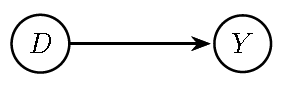
Figure 13.1: Directed Acyclic Graph (DAG) implied by a Randomized Controlled Trial (RCT).
The counterfactual representation of the DAG, known as the Single-World Intervention Graph (SWIG), is shown in the following figure. In this figure, the treatment variable \(D\) is split to reflect the intervention: we fix \(D\) at a specific value \(d\) (the intervention), and replace the outcome \(Y\) with its counterfactual representation \(Y(d)\), which denotes the value of \(Y\) if \(D\) were set to \(d\). The natural value of \(D\) is also shown but becomes irrelevant for the outcome once the intervention is imposed.
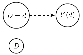
Figure 13.2: Single-World Intervention Graph (SWIG) for intervention \(do(D=d)\): \(Y\) is replaced by the counterfactual \(Y(d)\), and \(D\) is split into the fixed value \(D=d\) and its natural value \(D\). The dashed arrow indicates the fixed causal assignment.
Note that we can express the observed outcome in terms of the potential outcomes as: \[ Y_i = [Y_i(1) - Y_i(0)] D_i + Y_i(0), \] which shows that the observed outcome equals the control potential outcome plus the treatment effect if treated.
Under the assumption of a constant treatment effect and a linear Conditional Expectation Function (CEF) \(\mathbb{E}[Y_i\mid D_i]\), this relationship can be represented as a linear regression model (Angrist and Pischke 2009): \[ Y_i = \underbrace{\beta_0}_{\mathbb{E}[Y_i(0)]} + \underbrace{\tau}_{\text{constant treatment effect}} D_i + \underbrace{\mu_i}_{Y_i(0) - \mathbb{E}[Y_i(0)]}, \] where \(\tau\) represents the common treatment effect across all units.
Under random assignment, we have \[\begin{equation*} \mathbb{E}[\mu_i \mid D_i] = \mathbb{E}[Y_i(0) \mid D_i] - \mathbb{E}[Y_i(0)] = \mathbb{E}[Y_i(0)] - \mathbb{E}[Y_i(0)] = 0, \end{equation*}\]
that is, the error term is mean-independent of treatment status. This implies that a regression of \(Y_i\) on \(D_i\) consistently estimates the causal effect under random assignment.
Example: Simple example
Bayesian inference for causal effects in a completely randomized experiment without covariates can be illustrated using the normal model in Donald B. Rubin (1990). Assume that \(Y_i(d) \sim N(\mu_d, \sigma_d^2)\) for \(d \in \{1,0\}\). Then, the likelihood function given a random sample and independent treatment assignment is: \[\begin{align*} p(\mathbf{y} \mid \mathbf{d}; \mu_1,\mu_0,\sigma^2_1,\sigma^2_0) &= \prod_{i:d_i=1}\phi(y_i \mid \mu_1,\sigma_1^2) \prod_{i:d_i=0}\phi(y_i \mid \mu_0,\sigma_0^2) \\ &= \prod_{i}\phi(y_i \mid \mu_1,\sigma_1^2)^{d_i} \, \phi(y_i \mid \mu_0,\sigma_0^2)^{1-d_i}, \end{align*}\] where \(\mathbf{y}\) and \(\mathbf{d}\) collect the observations of the outcomes and treatments, and \(\phi(\cdot)\) denotes the normal density function.
Assume conjugate priors: \[ \mu_d \mid \sigma^2_d \sim N\left(\mu_{0d}, \frac{\sigma^2_d}{\beta_{0d}}\right), \qquad \sigma^2_d \sim IG\left(\frac{\alpha_{0d}}{2}, \frac{\delta_{0d}}{2}\right). \]
From the normal/inverse-gamma model in Chapter 3, the posterior conditional distributions are: \[ \mu_d \mid \sigma^2_d, \{y_i,d_i\}_{i:d_i=d} \sim N \left(\mu_{nd}, \frac{\sigma^2_d}{\beta_{nd}}\right), \] where \[ \mu_{nd} = \frac{\beta_{0d}\mu_{0d} + N_d \bar{y}_d}{\beta_{0d} + N_d}, \qquad \beta_{nd} = \beta_{0d} + N_d, \] \(\bar{y}_d\) and \(N_d\) denote the sample mean and sample size of group \(d\). For the variance: \[ \sigma^2_d \mid \{y_i,d_i\}_{i:d_i=d} \sim IG\left(\frac{\alpha_{nd}}{2}, \frac{\delta_{nd}}{2}\right), \] where \[ \alpha_{nd} = \alpha_{0d} + N_d, \qquad \delta_{nd} = \sum_{i:d_i=d} (y_i-\bar{y}_d)^2 + \delta_{0d} + \frac{\beta_{0d}N_d}{\beta_{0d}+N_d}(\bar{y}_d-\mu_{0d})^2. \]
In addition, the predictive distribution is given by \[ Y(d)\mid \mathbf{y}\sim t\left(\mu_{nd},\frac{(\beta_{nd}+1)\delta_{nd}}{\beta_{nd}\alpha_{nd}},\alpha_{nd}\right). \]
Therefore, given the definition of the average treatment effect, \[\begin{align*} \text{ATE} & = \mathbb{E}[Y(1) - Y(0)]\\ & = \mathbb{E}[Y(1)] - \mathbb{E}[Y(0)]\\ & = \int_{\mathcal{R}} y(1) f_{Y(1)}(y(1))dy(1) - \int_{\mathcal{R}} y(0) f_{Y(0)}(y(0))dy(0)\\ & = \mu_{1} - \mu_{0}. \end{align*}\]
Note that this expectation is taken with respect to the population distribution of the potential outcomes, not with respect to the posterior distribution.74 Thus, the posterior distribution of the ATE is given by \[ \pi(\text{ATE}\mid \mathbf{y}) = \pi(\mu_{1} - \mu_{0}\mid \mathbf{y}). \]
We can obtain this posterior distribution by simulation, because the difference of two independent Student’s \(t\)-distributed random variables does not follow a Student’s \(t\) distribution. However, as the degrees of freedom increase, each posterior distribution of \(\mu_{d}\) converges to a normal distribution, and the difference of two normals is also normal. Consequently, an approximate point estimate of the ATE is \(\mu_{n1} - \mu_{n0}\), which asymptotically equals \(\bar{y}_1 - \bar{y}_0\) under non-informative priors. This is the classical estimator of the ATE.
Finally, note that we can also obtain the posterior distribution of the ATE using the simple linear regression framework by assuming non-informative prior distributions, in which case the posterior mean of the slope parameter coincides with the maximum likelihood estimator (see Exercise 1).
Let’s assume that \(\mu_1 = 15\), \(\mu_0 = 10\), \(\sigma_1^2 = 4\), \(\sigma_0^2 = 2\), and \(N_1=N_0=100\), and compute the posterior distribution of the ATE. The following code illustrates this procedure, while the following figures display the predictive densities of the potential outcomes and the posterior distribution of the ATE. The posterior mean is 4.60, and the 95% credible interval is (4.10, 5.12). Note that the population value is \(\mu_1-\mu_0=5\).
set.seed(10101)
# Parameters
mu1 <- 15; mu0 <- 10
sigma1 <- sqrt(4); sigma0 <- sqrt(2)
N1 <- 100; N0 <- 100
# Simulate data
y1 <- rnorm(N1, mu1, sigma1); y0 <- rnorm(N0, mu0, sigma0)
# Prior hyperparameters
alpha0 <- 0.01; delta0 <- 0.01
simulate_t <- function(y) {
    N <- length(y); ybar <- mean(y)
    sse <- sum((y - ybar)^2)
    alpha_n <- alpha0 + N; delta_n <- sse + delta0
    scale2 <- ((N + 1) * delta_n) / (N * alpha_n)
    df <- alpha_n
    loc <- ybar; scale <- sqrt(scale2)
    rt(1, df = df) * scale + loc
}
# Posterior predictive draws
ppd1 <- replicate(1000, simulate_t(y1))
ppd0 <- replicate(1000, simulate_t(y0))
# Plot
hist(ppd1, col = rgb(1, 0, 0, 0.4), freq = FALSE, main = "Posterior Predictive",
xlab = "Y", xlim = c(5, 25))
hist(ppd0, col = rgb(0, 0, 1, 0.4), freq = FALSE, add = TRUE)
legend("topright", legend = c("Treatment", "Control"),
fill = c(rgb(1, 0, 0, 0.4), rgb(0, 0, 1, 0.4)))
# Posterior distribution of ATE
posterior_mu <- function(y) {
    N <- length(y); ybar <- mean(y)
    sse <- sum((y - ybar)^2)
    alpha_n <- alpha0 + N
    delta_n <- sse + delta0
    # Posterior variance for mean
    var_mu <- delta_n / (alpha_n * N)
    df <- alpha_n
    loc <- ybar; scale <- sqrt(var_mu)
    rt(1, df = df) * scale + loc
}
# Posterior draws for parameters
n_draws <- 10000
mu1_draws <- replicate(n_draws, posterior_mu(y1))
mu0_draws <- replicate(n_draws, posterior_mu(y0))
# Parameter uncertainty: difference of means
ate_draws <- mu1_draws - mu0_draws
summary(coda::mcmc(ate_draws))
##
## Iterations = 1:10000
## Thinning interval = 1
## Number of chains = 1
## Sample size per chain = 10000
##
## 1. Empirical mean and standard deviation for each variable,
## plus standard error of the mean:
##
## Mean SD Naive SE Time-series SE
## 4.607604 0.255213 0.002552 0.002552
##
## 2. Quantiles for each variable:
##
## 2.5% 25% 50% 75% 97.5%
## 4.100 4.440 4.604 4.778 5.117# Summaries
ate_mean <- mean(ate_draws)
ci <- quantile(ate_draws, c(0.025, 0.975))
cat("Posterior mean of ATE:", ate_mean, "\n")## Posterior mean of ATE: 4.607604## 95% Credible Interval: 4.100032 5.116916# Plot posterior distribution of ATE
hist(ate_draws, breaks = 50, freq = FALSE,
main = "Posterior Distribution of ATE",
xlab = "ATE (Y(1) - Y(0))", col = "lightblue", border = "white")
abline(v = ate_mean, col = "red", lwd = 2)
abline(v = ci, col = "darkgreen", lty = 2, lwd = 2)
legend("topright", legend = c("Posterior Mean", "95% Credible Interval"), col = c("red", "darkgreen"), lwd = 2, lty = c(1, 2), bty = "n", cex = 0.8) # Smaller legend using cex
An RCT is considered the gold standard for identifying causal effects because it provides the strongest basis for satisfying the key identification assumption in causal inference: independence between treatment assignment and potential outcomes. However, RCTs may face challenges such as non-compliance, which occurs when individuals do not adhere to their assigned treatment in an experimental study. This matters because, in many real-world settings, some individuals do not take the treatment they were assigned, leading to deviations from the ideal randomized controlled trial design. In addition, RCTs are sometimes infeasible due to ethical, logistical, or financial constraints. Moreover, they can be too narrowly focused or localized to provide general conclusions about what works (Deaton 2010). Thus, the external validity of causal effects from RCTs may be questionable.
It is also important to note that RCTs primarily identify the mean of the treatment effect distribution but do not capture other features, such as the median or higher-order moments. These additional aspects of the distribution of treatment effects can be highly relevant for policymakers and stakeholders. See Deaton (2010) for a detailed discussion of other potential shortcomings of RCTs.
References
Other functions of the potential outcomes, such as \(P(Y(1)\geq Y(0))\), require the joint distribution of the potential outcomes rather than just the marginal distributions, as is the case for the ATE.↩︎