13.6 Regression discontinuity design (RD)
In this section, we study the regression discontinuity (RD) design. In particular, we analyze the causal effect of a binary treatment \(D_i\) on an outcome \(Y_i\) within the potential outcomes (Rubin causal model) framework, namely \(Y_i(1)-Y_i(0)\). As usual, we face the fundamental problem of causal inference. Identification in RD relies on a running variable \(Z_i\), also known as the forcing, index, or score variable, which determines treatment assignment, either completely or partially, depending on whether a unit lies on either side of a known cutoff \(c\). The running variable may be associated with the potential outcomes, but this association is assumed to be smooth at \(c\). Under this smoothness assumption (and in the absence of precise manipulation at \(c\)), any discontinuity in the conditional mean of \(Y_i\) as a function of \(Z_i\) at \(c\) identifies the causal effect of the treatment at the cutoff (Guido W. Imbens and Lemieux 2008).
There are two common versions of RD: sharp and fuzzy. In the former, the change (jump) in the conditional probability of treatment at the cutoff equals one; in the latter, it is strictly between zero and one:
\[ \Delta \;=\; \lim_{z \downarrow c}\Pr(D_i=1\mid Z_i=z)-\lim_{z \uparrow c}\Pr(D_i=1\mid Z_i=z) = \begin{cases} 1, & \text{sharp RD},\\[2pt] \in(0,1), & \text{fuzzy RD}. \end{cases} \]
Here \(\lim_{z \downarrow c}\) and \(\lim_{z \uparrow c}\) denote the right (approach from above) and left (approach from below) limits, respectively.
13.6.1 Sharp regression discontinuity design (SRD)
In the sharp case, treatment assignment is a deterministic function of the running variable:
\[ D_i = \mathbf{1}\{Z_i \ge c\}, \]
so the conditional probability of treatment jumps from \(0\) to \(1\) at \(Z_i=c\). All units with \(Z_i \ge c\) are treated, whereas those with \(Z_i < c\) serve as the control group. Therefore, assignment is identical to treatment in the sharp RD (perfect compliance). The following figure displays the conditional probability of treatment.
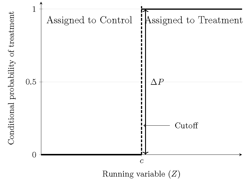
Figure 13.9: Sharp regression discontinuity design: Conditional probability of treatment.
The observed outcome is given by
\[ Y_i=(1-D_i)\cdot Y_i(0) + D_i\cdot Y_i(1)= \begin{cases} Y_i(0), & Z_i < c,\\ Y_i(1), & Z_i \geq c. \end{cases} \]
Thus, the causal effect that we target in SRD is
\[ \tau_{SRD}=\mathbb{E}[Y_i(1)-Y_i(0)\mid Z_i=c]. \]
Note that the treatment effect is evaluated at the cutoff, which is a single point in the support of the running variable. Hence \(\tau_{\text{SRD}}\) is inherently local and need not be representative of units whose running variable lies far from \(c\).
The identification of \(\tau_{\text{SRD}}\) requires continuity of the potential outcome regression functions, that is,
\[ \mathbb{E}[Y_i(0)\mid Z_i=z]\ \text{and}\ \mathbb{E}[Y_i(1)\mid Z_i=z] \]
are continuous at \(z\). Strictly speaking, it suffices that the left- and right-hand limits of \(\mathbb{E}[Y_i(d)\mid Z_i=z]\) coincide at \(z=c\) for \(d\in\{0,1\}\).
This implies
\[ \begin{aligned} \mathbb{E}[Y_i(0)\mid Z_i=c] &= \lim_{z \uparrow c}\mathbb{E}[Y_i(0)\mid Z_i=z] \\ &= \lim_{z \uparrow c}\mathbb{E}[Y_i(0)\mid Z_i=z, D_i=0] \\ &= \lim_{z \uparrow c}\mathbb{E}[Y_i\mid Z_i=z], \end{aligned} \]
since for \(z<c\) we have \(D_i=0\). Similarly,
\[ \begin{aligned} \mathbb{E}[Y_i(1)\mid Z_i=c] &= \lim_{z \downarrow c}\mathbb{E}[Y_i(1)\mid Z_i=z] \\ &= \lim_{z \downarrow c}\mathbb{E}[Y_i\mid Z_i=z], \end{aligned} \]
because for \(z>c\) we have \(D_i=1\). Therefore,
\[ \tau_{\text{SRD}} = \lim_{z \downarrow c}\mathbb{E}[Y_i\mid Z_i=z] - \lim_{z \uparrow c}\mathbb{E}[Y_i\mid Z_i=z], \]
i.e., the target estimand is the jump in the conditional mean at the discontinuity point \(c\). See the following figure.
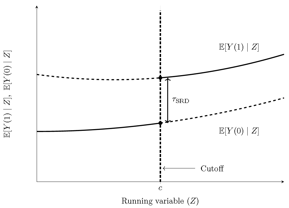
Figure 13.10: RD treatment effect in a sharp RD design. Solid segments are observed on each side of \(c\); dashed segments are counterfactual.
13.6.2 Fuzzy regression discontinuity design (FRD)
In the fuzzy case, the conditional probability of treatment has a discontinuous jump at the cutoff that is strictly between \(0\) and \(1\): \[\begin{align*} \lim_{z \uparrow c} \Pr(D_i=1 \mid Z_i=z) \ne \lim_{z \downarrow c} \Pr(D_i=1 \mid Z_i=z),\\ 0 \;<\; \lim_{z \downarrow c} \Pr(D_i=1 \mid Z_i=z) \;-\; \lim_{z \uparrow c} \Pr(D_i=1 \mid Z_i=z) \;<\; 1. \end{align*}\] Thus, the probability of treatment increases discontinuously at \(c\). Note that in a fuzzy RD, compliance is imperfect: some units assigned to treatment do not take it, and some units not assigned may nonetheless receive it. The following figure displays the conditional probability of treatment.
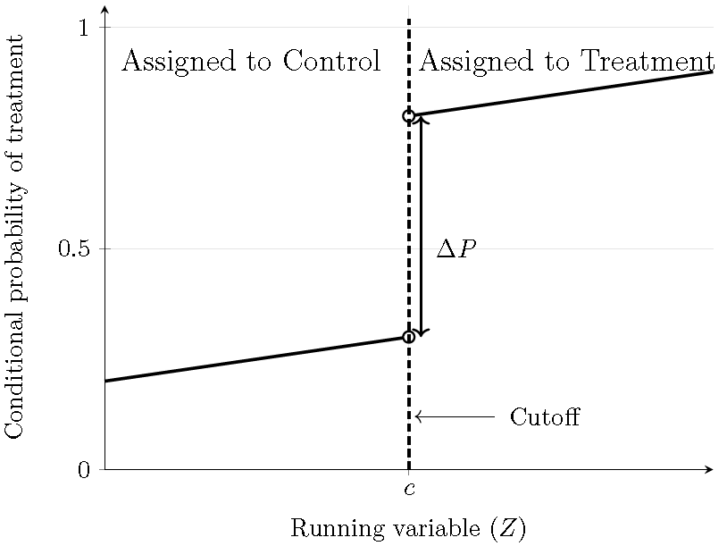
Figure 13.11: Fuzzy regression discontinuity design: Conditional probability of treatment.
Note that the expected value of the observed outcome given the running variable is given by \[\begin{align*} \mathbb{E}[Y_i\mid Z_i=z]&=\mathbb{E}[Y_i(0)\mid D_i=0, Z_i=z]P(D_i=0\mid Z_i=z)\\ &+\mathbb{E}[Y_i(1)\mid D_i=1, Z_i=z]P(D_i=1\mid Z_i=z). \end{align*}\]
Thus, the observed outcome is a weighted average of potential outcomes. The following figure displays the treatment effect that we are targeting.
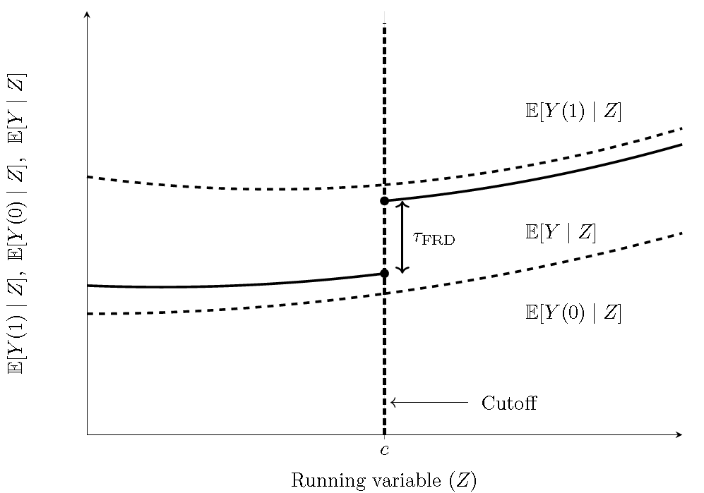
Figure 13.12: RD treatment effect in a fuzzy RD design. Solid segments are observed on each side of \(c\); dashed segments are counterfactual.
The target causal effect in the FRD is (see J. Hahn, Todd, and Klaauw (2001) for a proof)
\[ \tau_{\text{FRD}} = \frac{\lim_{z \downarrow c}\mathbb{E}[Y_i\mid Z_i=z]-\lim_{z \uparrow c}\mathbb{E}[Y_i\mid Z_i=z]} {\lim_{z \downarrow c}\mathbb{E}[D_i\mid Z_i=z]-\lim_{z \uparrow c}\mathbb{E}[D_i\mid Z_i=z]} = \mathbb{E}[Y_i(1)-Y_i(0)\mid Z_i=c], \ \text{units are compliers}. \]
Note that \(\tau_{\text{FRD}}\) encompasses \(\tau_{\text{SRD}}\) as \(\lim_{z \downarrow c}\mathbb{E}[D_i\mid Z_i=z]-\lim_{z \uparrow c}\mathbb{E}[D_i\mid Z_i=z]=1\) in the SRD. In addition, \(\tau_{\text{FRD}}\) has the same structure as the local average treatment effect (LATE) in the IV literature, with the instrument given by the eligibility indicator \(T_i=\mathbf{1}\{Z_i\ge c\}\). Because compliance is imperfect (some eligible units do not take treatment and some ineligible units receive it), \(D_i \neq T_i\) for some units, and the estimand pertains to compliers at the cutoff.
Let \(D_i(z)\) denote the potential treatment status if the cutoff were \(z\) (for \(z\) in a neighborhood of \(c\)) such that \(D_i(z)=1\) implies that the unit would be treated if the cutoff is \(z\). The identification assumptions are:
1. Continuity of the potential outcome regression functions, particularly at \(c\).
2. A nontrivial first stage,
\(\lim_{z \downarrow c}\mathbb{E}[D_i\mid Z_i=z]-\lim_{z \uparrow c}\mathbb{E}[D_i\mid Z_i=z]\neq 0\),
3. Monotonicity: \(D_i(z)\) is non-increasing in \(z\) at \(z=c\).
We can classify unit types (locally around the cutoff \(c\)) using the potential treatment under a hypothetical cutoff \(z\), \(D_i(z)\) as follows:
Complier status
\[
\lim_{z\downarrow Z_i}D_i(z)=0, \ \text{and} \ \lim_{z\uparrow Z_i}D_i(z)=1,
\]
Never-takers
\[
\lim_{z\downarrow Z_i}D_i(z)=0, \ \text{and} \ \lim_{z\uparrow Z_i}D_i(z)=0,
\]
Always-takers
\[
\lim_{z\downarrow Z_i}D_i(z)=1, \ \text{and} \ \lim_{z\uparrow Z_i}D_i(z)=1.
\]
Thus, compliers are units that would be treated if the cutoff were at or below their score \(Z_i\), and would not be treated if the cutoff were above \(Z_i\). Never-takers and always-takers do not change treatment status regardless of the cutoff: the former are always untreated, whereas the latter are always treated. Monotonicity precludes defiers.
See Guido W. Imbens and Lemieux (2008) and Cattaneo, Idrobo, and Titiunik (2019) for discussions of graphical and formal diagnostics of the assumptions in RD.
Example: Returns to compulsory schooling (Siddhartha Chib and Jacobi 2016)
Siddhartha Chib and Jacobi (2016) propose a Bayesian inferential framework that explicitly models unit type (complier, always-taker, and never-taker), which enables implementation of a Gibbs sampler. Their empirical application is motivated by the April 1947 reform in the United Kingdom that raised the minimum school-leaving age from 14 to 15.
In the example below, we construct a simulation calibrated to their application to illustrate Bayesian inference in a fuzzy RD. In particular, we specify priors, show the full conditional distributions, and implement a Gibbs sampler to estimate the treatment effect at the cutoff.
There are three types of individuals: compliers (\(c\)), never-takers (\(n\)), and always-takers (\(a\)). These imply four potential outcomes \(Y_{ic}(0)\), \(Y_{ic}(1)\), \(Y_{in}(0)\), and \(Y_{ia}(1)\). Siddhartha Chib and Jacobi (2016) assume
\[ Y_{ic}(0)=\beta_{0c0}+\beta_{0c1}Z_i+\mathbf{X}_i^{\top}\boldsymbol{\beta}_c+\mu_{0ci}=\mathbf{W}_{ic}^{\top}\beta_{0c}+\mu_{0ci}, \]
\[ Y_{ic}(1)=\beta_{1c0}+\beta_{1c1}Z_i+\mathbf{X}_i^{\top}\boldsymbol{\beta}_c+\mu_{1ci}=\mathbf{W}_{ic}^{\top}\beta_{1c}+\mu_{1ci}, \]
\[ Y_{in}(0)=\beta_{n0}+\mathbf{X}_i^{\top}\boldsymbol{\beta}_n+\mu_{ni}=\mathbf{W}_{in}^{\top}\beta_{0n}+\mu_{ni}, \]
and
\[ Y_{ia}(1)=\beta_{a0}+\mathbf{X}_i^{\top}\boldsymbol{\beta}_a+\mu_{ai}=\mathbf{W}_{ia}^{\top}\beta_{1a}+\mu_{ai}, \]
where \(\mu_{dci}\sim t_v(0,\sigma^2_{dc})\) for \(d\in\{0,1\}\), \(\mu_{ni}\sim t_v(0,\sigma^2_{0n})\), and \(\mu_{ai}\sim t_v(0,\sigma^2_{1a})\); here \(t_v\) denotes the Student-\(t\) distribution with \(v\) degrees of freedom. The running variable is centered at the cutoff, so \(Z_i=0\) at the threshold, and the FRD treatment effect is
\[ \tau_{\text{FRD}}=\beta_{1c0}-\beta_{0c0}. \]
There are four cells in this setting, defined by policy epochs \(\mathbf{1}(Z_i < 0)\) and \(\mathbf{1}(Z_i \geq 0)\), and treatment values \(D_i = 0\) and \(D_i = 1\). Table 13.5 shows the case where, in the cell without treatment under the old policy (\(K_{00}\)), there are compliers and never-takers, while in the cell with treatment under the new policy (\(K_{11}\)), there are compliers and always-takers.
| Policy indicator | \(D_i = 0\) | \(D_i = 1\) |
|---|---|---|
| \(\mathbf{1}(Z_i < 0)\) (old policy) | c, n | a |
| \(\mathbf{1}(Z_i \geq 0)\) (new policy) | n | c, a |
The four cells by policy and treatment status are:
\[ K_{00} = \{c, n\}, \quad K_{10} = \{n\}, \quad K_{01} = \{a\}, \quad K_{11} = \{c, a\}, \]
and the two cells by treatment status are:
\[ K_0 = \{c, n\}, \quad K_1 = \{c, a\}. \]
Under a Bayesian framework, posterior simulation simplifies because we sample each unit’s latent type \(C_i \in \{c, n, a\}\). This contrasts with the Frequentist literature, where types are not modeled explicitly. Thus, the Bayesian approach requires setting assumptions about the types (see Siddhartha Chib and Jacobi (2016) for details); for instance, types may be distributed smoothly around the cutoff with unknown distributions. In addition, given monotonicity, there are models for four potential outcomes. This differs from the Frequentist literature, which considers only two potential outcomes, given the binary treatment, and a model for the treatment.
Note that if we observe \(Z_i < 0\) and \(D_i = 0\), only compliers and never-takers are possible. Then,
\[ P(C_i = c \mid Y_i, D_i = 0, \boldsymbol{\theta}) = \frac{\eta_{c} \, t_v\!\big(Y_i \mid \mathbf{W}_{ic}^{\top} \boldsymbol{\beta}_{0c}, \sigma^2_{0c} \big)} {\eta_{c} \, t_v\!\big(Y_i \mid \mathbf{W}_{ic}^{\top} \boldsymbol{\beta}_{0c}, \sigma^2_{0c} \big) + \eta_{n} \, t_v\!\big(Y_i \mid \mathbf{W}_{in}^{\top} \boldsymbol{\beta}_{0n}, \sigma^2_{0n} \big)}, \quad i \in K_{00} \]
where \(\boldsymbol{\theta}\) denotes the set of model parameters, and \(\eta_{c}\) and \(\eta_{n}\) are the current mixture weights for a complier and a never-taker, respectively.
Conversely, if \(Z_i \geq 0\) and \(D_i = 1\), only compliers and always-takers are possible:
\[ P(C_i = c \mid Y_i, D_i = 1, \boldsymbol{\theta}) = \frac{\eta_{c} \, t_v\!\big(Y_i \mid \mathbf{W}_{ic}^{\top} \boldsymbol{\beta}_{1c}, \sigma^2_{1c} \big)} {\eta_{c} \, t_v\!\big(Y_i \mid \mathbf{W}_{ic}^{\top} \boldsymbol{\beta}_{1c}, \sigma^2_{1c} \big) + \eta_{a} \, t_v\!\big(Y_i \mid \mathbf{W}_{ia}^{\top} \boldsymbol{\beta}_{1a}, \sigma^2_{1a} \big)}, \quad i \in K_{11} \]
where \(\eta_{a}\) is the mixture weight for an always-taker.
Following Siddhartha Chib and Jacobi (2016), we assume a Dirichlet prior for the mixing probabilities (\(\eta_c, \eta_n,\eta_a\)) with hyperparameters \(\alpha_{0k}\), \(k \in \{c, n, a\}\). The posterior distribution is then Dirichlet with parameters \(\alpha_{0k} + \sum_{i=1}^N \mathbf{1}(C_i = k)\).
In addition, Siddhartha Chib and Jacobi (2016) use the normal–gamma mixture representation of the Student-\(t\) distribution, where the mixing parameter satisfies \(\lambda_i \sim G(v/2, v/2)\). Consequently, the posterior distribution of \(\lambda_i\) is gamma with parameters \((v+1)/2\) and \((v + \sigma_{dk}^{-2}(y_i - \mathbf{W}_{ik}^{\top} \boldsymbol{\beta}_{dk})^2) / 2\).
The prior distribution for the location parameters \(\boldsymbol{\beta}_{dk}\) is independent normal with mean \(\boldsymbol{\beta}_{dk,0}\) and variance matrix \(\mathbf{B}_{dk,0}\). The posterior distribution of \(\boldsymbol{\beta}_{dk}\) is normal with mean
\[ \boldsymbol{\beta}_{dk,n} = \mathbf{B}_{dk,n} \left( \mathbf{B}_{dk,0}^{-1} \boldsymbol{\beta}_{dk,0} + \sigma_{dk}^{-2} \sum_{i \in I_{dk}} \lambda_i \mathbf{W}_{ik} Y_i \right), \]
and covariance matrix
\[ \mathbf{B}_{dk,n} = \left( \mathbf{B}_{dk,0}^{-1} + \sigma_{dk}^{-2} \sum_{i \in I_{dk}} \lambda_i \mathbf{W}_{ik} \mathbf{W}_{ik}^{\top} \right)^{-1}, \]
where \(I_{dk} = \{i : D_i = d, C_i = k\}\) is the set of indices for observations by treatment status and unit type. Note that there are only four possible combinations determined by policy and treatment status, namely, \(I_{0c}\), \(I_{1c}\), \(I_{0n}\) and \(I_{1a}\).
Finally, assuming that the prior distributions of the variances are independent inverse-gamma, \(\sigma_{dk}^2 \sim IG(\alpha_{dk,0}/2, \delta_{dk,0}/2)\), the posterior distributions are also inverse-gamma, \(\sigma_{dk}^2 \sim IG(\alpha_{dk,n}/2, \delta_{dk,n}/2)\), where
\[ \alpha_{dk,n} = \alpha_{dk,0} + N_{dk}, \]
and
\[ \delta_{dk,n} = \delta_{dk,0} + \sum_{i \in I_{dk}} \lambda_i \left(Y_i - \mathbf{w}_{ik}^{\top} \boldsymbol{\beta}_{dk} \right)^2. \]
Here, \(N_{dk}\) denotes the number of elements (cardinality) of \(I_{dk}\).
The following code performs a simulation assuming that \(Z_i\) follows a discrete uniform distribution from \(-24\) to \(24\), where the policy indicator equals one if \(Z_i \geq 0\). Next, \(X_i\) follows a discrete uniform distribution between \(85\) and \(95\). We set \(\boldsymbol{\beta}_{0c} = [4.50 \ -0.20 \ 0.03]^{\top}\) and \(\boldsymbol{\beta}_{1c} = [5.50 \ 0.40 \ 0.03]^{\top}\), so that the treatment effect is \(1\). In addition, \(\boldsymbol{\beta}_{0n} = [6.80 \ -0.02]^{\top}\) and \(\boldsymbol{\beta}_{1a} = [5.50 \ -0.04]^{\top}\), with \(\sigma_{0c}^2 = \sigma_{1c}^2 = 0.10\), \(\sigma_{0n}^2 = 0.15\), and \(\sigma_{1a}^2 = 0.20\). The type probabilities are \(\eta_{c} = 0.70\), \(\eta_{n} = 0.15\), and \(\eta_{a} = 0.15\). We set the sample size to \(3{,}000\) and \(v = 5\). In addition, we set non-informative priors, a burn-in of 1,000, and 5,000 MCMC iterations. The following code illustrates the implementation, and the figure presents the posterior distribution of the LATE. The 95% credible interval encompasses the population value, and the posterior mean lies close to this value.
rm(list = ls()); set.seed(10101); library(ggplot2)
# Simulation setup
N <- 3000
Zi <- sample(seq(-24, 24, 1), N, replace = TRUE) # Running var
Z <- Zi - mean(Zi)
T <- as.integer(Z >= 0)                          # Policy (0/1)
X <- sample(seq(85, 95, 1), N, replace = TRUE)   # Regressor
Wc <- cbind(1, Z, X)                             # Compliers
W  <- cbind(1, X)                                # No compliers

B0c <- c(4.5, -0.2, 0.03); B1c <- c(5.5, 0.4,  0.03)
B0n <- c(6.8,  -0.02); B1a <- c(5.5,  -0.04)
s2c <- 0.1; s2n <- 0.15; s2a <- 0.2
Etac <- 0.7; Etan <- 0.15; Etaa <- 0.15
v <- 5
# Potential outcomes (Student-t noise scaled to match variances)
mu0c <- sqrt(s2c) * rt(N, v);  Y0c <- as.numeric(Wc %*% B0c + mu0c)
mu1c <- sqrt(s2c) * rt(N, v);  Y1c <- as.numeric(Wc %*% B1c + mu1c)
mu0n <- sqrt(s2n) * rt(N, v);  Y0n <- as.numeric(W  %*% B0n + mu0n)
mu1a <- sqrt(s2a) * rt(N, v);  Y1a <- as.numeric(W  %*% B1a + mu1a)
# Latent types: first n, then a, remaining are c
id    <- seq_len(N)
n_n   <- as.integer(round(Etan * N))
n_a   <- as.integer(round(Etaa * N))
id0n  <- sample(id, n_n, replace = FALSE)     # never-takers
id_rem <- setdiff(id, id0n)
id1a  <- sample(id_rem, n_a, replace = FALSE) # always-takers
idc   <- setdiff(id, c(id0n, id1a))           # compliers
type <- rep(NA_character_, N)
type[id0n] <- "n"
type[id1a] <- "a"
type[idc]  <- "c"
# Realized treatment under monotonicity:
# n -> D=0, a -> D=1, c -> D=T
D <- integer(N)
D[type == "n"] <- 0; D[type == "a"] <- 1
D[type == "c"] <- T[type == "c"]

# 2x2 table of D vs T
tab_DT <- table(T = factor(T, levels = 0:1), D = factor(D, levels = 0:1))
print(tab_DT)
## D
## T 0 1
## 0 1248 229
## 1 236 1287Y <- ifelse(type == "n", Y0n, ifelse(type == "a", Y1a, ifelse(D == 0, Y0c, Y1c)))
## Gibbs sampler ##
I00 <- which(T == 0 & D == 0); I11 <- which(T == 1 & D == 1)
I01 <- which(T == 0 & D == 1); I10 <- which(T == 1 & D == 0)
# Hyperparameters
a0c <- 1; a0n <- 1; a0a <- 1 # Hyperpar Dirichlet
v <- 5 # Student-t
a0 <- 0.01; d0 <- 0.01 # Inv-Gamma
# Prob complier | D=0
dens_t_locscale <- function(y, mu, sig2, v) {
z <- (y - mu) / sqrt(sig2); dt(z, df = v) / sqrt(sig2)
}
Pc0 <- function(b0c, sigma20c, etac, b0n, sigma20n, etan, i){
p0c <- etac * dens_t_locscale(Y[i], mu = sum(Wc[i,]*b0c), sig2 = sigma20c, v = v)
p0n <- etan * dens_t_locscale(Y[i], mu = sum(W[i, ]*b0n), sig2 = sigma20n, v = v)
pc0 <- p0c / (p0c + p0n + 1e-12)
return(pc0)
}
Pc1 <- function(b1c, sigma21c, etac, b1a, sigma21a, etaa, i){
p1c <- etac * dens_t_locscale(Y[i], mu = sum(Wc[i,]*b1c), sig2 = sigma21c, v = v)
p1a <- etaa * dens_t_locscale(Y[i], mu = sum(W[i, ]*b1a), sig2 = sigma21a, v = v)
pc1 <- p1c / (p1c + p1a + 1e-12)
return(pc1)
}
rtype <- function(alphas){
types <- MCMCpack::rdirichlet(1, alphas)
return(types)
}
PostLambda_i <- function(sig2, Beta, yi, hi, v){
shape <- (v + 1)/2
rate <- (v + (yi - sum(hi * Beta))^2 / sig2)/2
rgamma(1, shape = shape, rate = rate)
}
PostBeta <- function(sig2, lambda, y, H){
k <- dim(H)[2]; B0i <- solve(1000*diag(k))
b0 <- rep(0, k)
Bn <- solve(B0i + sig2^(-1)*t(H)%*%diag(lambda)%*%H)
bn <- Bn%*%(B0i%*%b0 + sig2^(-1)*t(H)%*%diag(lambda)%*%y)
Beta <- MASS::mvrnorm(1, bn, Bn)
return(Beta)
}
PostSig2 <- function(Beta, lambda, y, H){
Ndk <- length(y); an <- a0 + Ndk
dn <- d0 + t(y - H%*%Beta)%*%diag(lambda)%*%(y - H%*%Beta)
sig2 <- invgamma::rinvgamma(1, shape = an/2, rate = dn/2)
return(sig2)
}
# MCMC parameter
burnin <- 1000; S <- 5000; tot <- S + burnin
ETAs <- matrix(NA, tot, 3)
BETAS0C <- matrix(NA, tot, 3); BETAS1C <- matrix(NA, tot, 3)
BETASA <- matrix(NA, tot, 2); BETASN <- matrix(NA, tot, 2)
SIGMAS <- matrix(NA, tot, 4)
b0c <- rep(0, 3); b1c <- rep(0, 3); b1a <- rep(0, 2); b0n <- rep(0, 2)
sigma21c <- 0.1; sigma20c <- 0.1; sigma20n <- 0.1; sigma21a <- 0.1
EtacNew <- 0.5; EtanNew <- 0.25; EtaaNew <- 0.25
pb <- txtProgressBar(min = 0, max = tot, style = 3)## | | | 0%for(s in 1:tot){
ProbC0 <- sapply(I00, function(i)Pc0(b0c, sigma20c, EtacNew, b0n, sigma20n, EtanNew, i = i))
ProbC1 <- sapply(I11, function(i)Pc1(b1c, sigma21c, EtacNew, b1a, sigma21a, EtaaNew, i = i))
Typec0 <- sapply(ProbC0, function(p) {sample(c("c", "n"), 1, prob = c(p, 1-p))})
Typec1 <- sapply(ProbC1, function(p) {sample(c("c", "a"), 1, prob = c(p, 1-p))})
typeNew <- rep(NA_character_, N)
typeNew[I10] <- "n"; typeNew[I01] <- "a"
typeNew[I00] <- Typec0; typeNew[I11] <- Typec1
Nc <- sum(typeNew == "c"); Na <- sum(typeNew == "a")
Nn <- sum(typeNew == "n");
anc <- a0c + Nc; ann <- a0n + Nn; ana <- a0a + Na
alphas <- c(anc, ann, ana)
EtasNew <- rtype(alphas = alphas)
EtacNew <- EtasNew[1]; EtanNew <- EtasNew[2]
EtaaNew <- EtasNew[3]
ETAs[s, ] <- EtasNew; Lambda <- numeric(N)
idx_n <- which(typeNew == "n")
idx_a <- which(typeNew == "a")
idx_c0 <- which(typeNew == "c" & D == 0); idx_c1 <- which(typeNew == "c" & D == 1)
Lambda[idx_n] <- sapply(idx_n, function(i) PostLambda_i(sigma20n, b0n, Y[i], W[i, ], v))
Lambda[idx_a] <- sapply(idx_a, function(i) PostLambda_i(sigma21a, b1a, Y[i], W[i, ], v))
Lambda[idx_c0] <- sapply(idx_c0, function(i) PostLambda_i(sigma20c, b0c, Y[i], Wc[i, ], v))
Lambda[idx_c1] <- sapply(idx_c1, function(i) PostLambda_i(sigma21c, b1c, Y[i], Wc[i, ], v))
b1a <- PostBeta(sig2 = sigma21a, lambda = Lambda[idx_a], y = Y[idx_a], H = W[idx_a,])
b0n <- PostBeta(sig2 = sigma20n, lambda = Lambda[idx_n], y = Y[idx_n], H = W[idx_n,])
b0c <- PostBeta(sig2 = sigma20c, lambda = Lambda[idx_c0], y = Y[idx_c0], H = Wc[idx_c0,])
b1c <- PostBeta(sig2 = sigma21c, lambda = Lambda[idx_c1], y = Y[idx_c1], H = Wc[idx_c1,])
BETASA[s, ] <- b1a; BETASN[s, ] <- b0n
BETAS0C[s, ] <- b0c; BETAS1C[s, ] <- b1c
sigma21a <- PostSig2(Beta = b1a, lambda = Lambda[idx_a], y = Y[idx_a], H = W[idx_a,])
sigma20n <- PostSig2(Beta = b0n, lambda = Lambda[idx_n], y = Y[idx_n], H = W[idx_n,])
sigma20c <- PostSig2(Beta = b0c, lambda = Lambda[idx_c0], y = Y[idx_c0], H = Wc[idx_c0,])
sigma21c <- PostSig2(Beta = b1c, lambda = Lambda[idx_c1], y = Y[idx_c1], H = Wc[idx_c1,])
SIGMAS[s, ] <- c(sigma21a, sigma20n, sigma20c, sigma21c)
setTxtProgressBar(pb, s)
}## | | | 1% | |= | 1% | |= | 2% | |== | 2% | |== | 3% | |== | 4% | |=== | 4% | |=== | 5% | |==== | 5% | |==== | 6% | |===== | 6% | |===== | 7% | |===== | 8% | |====== | 8% | |====== | 9% | |======= | 9% | |======= | 10% | |======= | 11% | |======== | 11% | |======== | 12% | |========= | 12% | |========= | 13% | |========= | 14% | |========== | 14% | |========== | 15% | |=========== | 15% | |=========== | 16% | |============ | 16% | |============ | 17% | |============ | 18% | |============= | 18% | |============= | 19% | |============== | 19% | |============== | 20% | |============== | 21% | |=============== | 21% | |=============== | 22% | |================ | 22% | |================ | 23% | |================ | 24% | |================= | 24% | |================= | 25% | |================== | 25% | |================== | 26% | |=================== | 26% | |=================== | 27% | |=================== | 28% | |==================== | 28% | |==================== | 29% | |===================== | 29% | |===================== | 30% | |===================== | 31% | |====================== | 31% | |====================== | 32% | |======================= | 32% | |======================= | 33% | |======================= | 34% | |======================== | 34% | |======================== | 35% | |========================= | 35% | |========================= | 36% | |========================== | 36% | |========================== | 37% | |========================== | 38% | |=========================== | 38% | |=========================== | 39% | |============================ | 39% | |============================ | 40% | |============================ | 41% | |============================= | 41% | |============================= | 42% | |============================== | 42% | |============================== | 43% | |============================== | 44% | |=============================== | 44% | |=============================== | 45% | |================================ | 45% | |================================ | 46% | |================================= | 46% | |================================= | 47% | |================================= | 48% | |================================== | 48% | |================================== | 49% | |=================================== | 49% | |=================================== | 50% | |=================================== | 51% | |==================================== | 51% | |==================================== | 52% | |===================================== | 52% | |===================================== | 53% | |===================================== | 54% | |====================================== | 54% | |====================================== | 55% | |======================================= | 55% | |======================================= | 56% | |======================================== | 56% | |======================================== | 57% | |======================================== | 58% | |========================================= | 58% | |========================================= | 59% | |========================================== | 59% | |========================================== | 60% | |========================================== | 61% | |=========================================== | 61% | |=========================================== | 62% | |============================================ | 62% | |============================================ | 63% | |============================================ | 64% | |============================================= | 64% | |============================================= | 65% | |============================================== | 65% | |============================================== | 66% | |=============================================== | 66% | |=============================================== | 67% | |=============================================== | 68% | |================================================ | 68% | |================================================ | 69% | |================================================= | 69% | |================================================= | 70% | |================================================= | 71% | |================================================== | 71% | |================================================== | 72% | |=================================================== | 72% | |=================================================== | 73% | |=================================================== | 74% | |==================================================== | 74% | |==================================================== | 75% | |===================================================== | 75% | |===================================================== | 76% | |====================================================== | 76% | |====================================================== | 77% | |====================================================== | 78% | |======================================================= | 78% | |======================================================= | 79% | |======================================================== | 79% | |======================================================== | 80% | |======================================================== | 81% | |========================================================= | 81% | |========================================================= | 82% | |========================================================== | 82% | |========================================================== | 83% | |========================================================== | 84% | |=========================================================== | 84% | |=========================================================== | 85% | |============================================================ | 85% | |============================================================ | 86% | |============================================================= | 86% | |============================================================= | 87% | |============================================================= | 88% | |============================================================== | 88% | |============================================================== | 89% | |=============================================================== | 89% | |=============================================================== | 90% | |=============================================================== | 91% | |================================================================ | 91% | |================================================================ | 92% | |================================================================= | 92% | |================================================================= | 93% | |================================================================= | 94% | |================================================================== | 94% | |================================================================== | 95% | |=================================================================== | 95% | |=================================================================== | 96% | |==================================================================== | 96% | |==================================================================== | 97% | |==================================================================== | 98% | |===================================================================== | 98% | |===================================================================== | 99% | |======================================================================| 99% | |======================================================================| 100%keep <- seq((burnin+1), tot)
LATE <- coda::mcmc(BETAS1C[keep, 1] - BETAS0C[keep, 1])
# Extract samples as numeric
late_draws <- as.numeric(LATE)
# Posterior mean and 95% CI
LATEmean <- mean(late_draws)
LATEci <- quantile(late_draws, c(0.025, 0.975))
# Plot posterior density
df <- data.frame(LATE = late_draws)
ggplot(df, aes(x = LATE)) + geom_density(fill = "skyblue", alpha = 0.5, color = "blue") + geom_vline(xintercept = LATEmean, color = "red", linetype = "dashed", linewidth = 1) + geom_vline(xintercept = LATEci, color = "black", linetype = "dotted", linewidth = 1) + labs(title = "Posterior distribution of LATE",
subtitle = paste0("Mean = ", round(LATEmean,3), " | 95% CI = [", round(LATEci[1],3), ", ", round(LATEci[2],3), "]"), x = "LATE", y = "Density") +
theme_bw(base_size = 14)
A difference in this example is that, unlike most of the Frequentist literature, the entire dataset on the forcing variable is used. Siddhartha Chib, Greenberg, and Simoni (2023) propose a non-parametric Bayesian framework that emphasizes the data near the cutoff using a soft-window approach. Other Bayesian approaches to inference in RD include Branson et al. (2019), who use Gaussian process regression to model the conditional expectation function, and Rischard et al. (2020), who develop a non-parametric Bayesian framework for spatial RD.