13.8 Bayesian exponentially tilted empirical likelihood
Bayesian parametric approaches are often criticized because they require distributional assumptions that may be arbitrary or remain unchecked. For example, in this chapter we model a continuous outcome as normally distributed. This choice is defensible: among all distributions with a fixed mean and variance, the normal imposes the least prior structure (it maximizes entropy; see Exercise 2), and the same reasoning extends to regression via Gaussian errors with fixed conditional variance (Zellner 1996a). Nevertheless, in some settings it may be preferable to use partial information methods that rely only on moment conditions rather than full distributional assumptions. The trade-off is familiar: unless the parametric model is correctly specified, these semiparametric approaches typically reduce efficiency relative to a well-specified parametric model.
The point of departure is a set of moment conditions
\[ \mathbb{E}\!\big[\mathbf{g}(\mathbf{W},\boldsymbol{\theta})\big]=\mathbf{0}_{d}, \]
where the expectation is with respect to the population distribution, \(\mathbf{W}_{1:N}:=[\mathbf{W}_1 \ \mathbf{W}_2 \ \dots \ \mathbf{W}_N]\) is a random sample from \(\mathbf{W}\subset \mathbb{R}^{d_w}\), \(\mathbf{g}:\mathbb{R}^{d_w}\times\boldsymbol{\Theta}\to\mathbb{R}^{d}\) is a vector of known functions, and \(\boldsymbol{\theta}=[\theta_{1}\ \theta_{2}\ \dots\ \theta_{p}]^{\top}\in\boldsymbol{\Theta}\subset\mathbb{R}^{p}\). If \(d>p\) the model is over-identified; if \(d=p\) it is exactly identified (and if \(d<p\) it is under-identified).
Example: Linear regression
Let
\[ y_i=\mathbf{X}_i^{\top}\boldsymbol{\beta}+\mu_i,\qquad \mathbb{E}[\mu_i\mid \mathbf{X}_i]=0, \]
with \(\mathbf{X}_i\in\mathbb{R}^{p}\) and \(\boldsymbol{\beta}\in\mathbb{R}^{p}\). Then the unconditional moment conditions are
\[ \mathbb{E}\!\left[\mathbf{X}_i\,\mu_i\right] =\mathbb{E}\!\left[\mathbf{X}_i\,(y_i-\mathbf{X}_i^{\top}\boldsymbol{\beta})\right] =\mathbf{0}_{p}. \]
Example: Instrumental variables
If there is endogeneity, \(\mathbb{E}[\mu_i\mid \mathbf{X}_i]\neq 0\), but there exist instruments \(\mathbf{Z}_i\in\mathbb{R}^{d}\) that are exogenous, \(\mathbb{E}[\mu_i\mid \mathbf{Z}_i]=0\), and relevant, \(\operatorname{rank}\!\big(\mathbb{E}[\mathbf{Z}_i\mathbf{X}_i^{\top}]\big)=p\), then
\[ \mathbb{E}\!\left[\mathbf{Z}_i\,\mu_i\right] =\mathbb{E}\!\left[\mathbf{Z}_i\,(y_i-\mathbf{X}_i^{\top}\boldsymbol{\beta})\right] =\mathbf{0}_{d}, \]
with \(d\ge p\).
Moment conditions can be used in a Bayesian framework via Bayesian Empirical Likelihood (BEL) (Nicole A. Lazar 2003) and Bayesian Exponentially Tilted Empirical Likelihood (BETEL) (Schennach 2005). We focus on BETEL because, while BEL inherits the attractive properties of empirical likelihood under correct specification, it can lose them under model misspecification. In contrast, Exponentially Tilted Empirical Likelihood (ETEL) remains well behaved under misspecification and retains root-\(N\) consistency and asymptotic normality (Schennach 2007).
Thus, the posterior distribution is
\[ \pi(\boldsymbol{\theta}\mid \mathbf{W}_{1:N}) \;\propto\; \pi(\boldsymbol{\theta})\; L_{\mathrm{ETEL}}(\boldsymbol{\theta}), \qquad L_{\mathrm{ETEL}}(\boldsymbol{\theta})=\prod_{i=1}^N p_i^{*}(\boldsymbol{\theta}), \]
where \(\pi(\boldsymbol{\theta})\) is the prior and \(L_{\mathrm{ETEL}}\) is the exponentially tilted empirical likelihood. The weights \(\big(p_1^{*}(\boldsymbol{\theta}),\dots,p_N^{*}(\boldsymbol{\theta})\big)\) are obtained from the maximum-entropy problem
\[ \max_{\{p_i\}_{i=1}^N}\;\Big\{-\sum_{i=1}^N p_i\log p_i\Big\} \quad\text{subject to}\quad \sum_{i=1}^N p_i=1,\;\; p_i\ge 0,\;\; \sum_{i=1}^N p_i\,\mathbf{g}(\mathbf{W}_i,\boldsymbol{\theta})=\mathbf{0}_d. \]
Equivalently (dual/saddlepoint form; see Schennach (2005);Schennach (2007);Siddhartha Chib, Shin, and Simoni (2018)),
\[ p_i^{*}(\boldsymbol{\theta}) =\frac{\exp\!\big(\boldsymbol{\lambda}(\boldsymbol{\theta})^{\top}\mathbf{g}(\mathbf{W}_i,\boldsymbol{\theta})\big)} {\sum_{j=1}^N \exp\!\big(\boldsymbol{\lambda}(\boldsymbol{\theta})^{\top}\mathbf{g}(\mathbf{W}_j,\boldsymbol{\theta})\big)}, \quad\text{where}\quad \sum_{i=1}^N p_i^{*}(\boldsymbol{\theta})\,\mathbf{g}(\mathbf{W}_i,\boldsymbol{\theta})=\mathbf{0}_d. \]
\(\boldsymbol{\lambda}(\boldsymbol{\theta})\) can be characterized as
\[ \boldsymbol{\lambda}(\boldsymbol{\theta}) =\arg\min_{\boldsymbol{\lambda}\in\mathbb{R}^{d}} \;\log\!\left(\frac{1}{N}\sum_{i=1}^N \exp\!\big(\boldsymbol{\lambda}^{\top}\mathbf{g}(\mathbf{W}_i,\boldsymbol{\theta})\big)\right), \]
whose gradient condition is precisely the moment constraint above. Therefore, the BETEL posterior is
\[ \pi(\boldsymbol{\theta}\mid \mathbf{w}_{1:N}) \;\propto\; \pi(\boldsymbol{\theta})\; \prod_{i=1}^N \frac{\exp\!\big(\boldsymbol{\lambda}(\boldsymbol{\theta})^{\top}\mathbf{g}(\mathbf{W}_i,\boldsymbol{\theta})\big)} {\sum_{j=1}^N \exp\!\big(\boldsymbol{\lambda}(\boldsymbol{\theta})^{\top}\mathbf{g}(\mathbf{W}_j,\boldsymbol{\theta})\big)}. \]
Posterior inference of the BETEL can be performed using a Metropolis-Hastings algorithm where the proposal distribution is \(q(\boldsymbol{\theta}\mid \mathbf{W}_{1:N})\). See the following algorithm (Siddhartha Chib, Shin, and Simoni 2018).
Algorithm: Bayesian Exponentially Tilted Empirical Likelihood (BETEL) – Metropolis–Hastings
Let \(W_{1:N} = \{W_1,\dots,W_N\}\) denote the sample.
Initialization:
Choose an initial value
\[ \theta^{(0)} \in \text{supp}\!\left\{ \pi(\theta \mid W_{1:N}) \right\}. \]Metropolis–Hastings iterations: For \(s = 1,2,\ldots,S\):
Proposal step:
Draw a candidate value
\[ \theta^{c} \sim q(\theta \mid W_{1:N}). \]Compute empirical likelihood weights:
Solve for \(p_{i}^{*}(\theta^{c})\), \(i = 1,\ldots,N\),
using the BETEL tilting equation that defines the Lagrange multiplier \(\lambda\).Acceptance probability:
\[ \alpha\big(\theta^{(s-1)}, \theta^{c} \mid W_{1:N}\big) = \min\!\left\{ 1,\; \frac{ \pi\!\left(\theta^{c} \mid W_{1:N}\right) }{ \pi\!\left(\theta^{(s-1)} \mid W_{1:N}\right) } \times \frac{ q\!\left(\theta^{(s-1)} \mid W_{1:N}\right) }{ q\!\left(\theta^{c} \mid W_{1:N}\right) } \right\}. \]Accept–reject step:
Draw \(U \sim \text{Uniform}(0,1)\) and set
\[ \theta^{(s)} = \begin{cases} \theta^{c}, & \text{if } U \leq \alpha\big(\theta^{(s-1)}, \theta^{c} \mid W_{1:N}\big), \\[6pt] \theta^{(s-1)}, & \text{otherwise}. \end{cases} \]
End for.
Example: Classical measurement error in regressor
Let’s set the unobserved (latent) regressor \(X_i^*\) such that
\[ X_i = X_i^* + \nu_i, \]
where \(X_i\) is the observed regressor, and \(\nu_i\) is a classical measurement error such that \(\mathbb{E}[\nu_i]=0\) and \(\nu_i \perp \{X_i^*,\mu_i\}\), where \(\mu_i\) is the stochastic error of the structural model
\[ Y_i=\beta_0+\beta_1X_i^*+\mu_i, \]
where \(\mathbb{E}[\mu_i]=0\) and \(\mu_i\perp X_i^*\).
If we perform the regression using the observed regressor, then
\[ Y_i=\beta_0+\beta_1(X_i-\nu_i)+\mu_i =\beta_0+\beta_1X_i+\underbrace{\mu_i-\beta_1\nu_i}_{\epsilon_i}, \]
where the new error term is \(\epsilon_i=\mu_i-\beta_1\nu_i\). We will show that
\[ \mathbb{E}[\epsilon_i\mid X_i]\neq 0. \]
By the law of iterated expectations,
\[ \mathbb{E}[\nu_i X_i] = \mathbb{E}\!\left[X_i \, \mathbb{E}[\nu_i \mid X_i]\right]. \]
This implies:
If \(\mathbb{E}[\nu_i \mid X_i] = 0\) almost surely, then \(\mathbb{E}[\nu_i X_i] = 0\).
If \(\mathbb{E}[\nu_i X_i] \neq 0\), then \(\mathbb{E}[\nu_i \mid X_i]\) cannot be equal to zero almost surely.
Now compute
\[ \mathbb{E}[\nu_iX_i] = \mathbb{E}[\nu_i(X_i^*+\nu_i)] = \underbrace{\mathbb{E}[\nu_i X_i^*]}_{=0} + \mathbb{E}[\nu_i^2] = \sigma^2_{\nu} \neq 0. \]
Hence it must be that \(\mathbb{E}[\nu_i\mid X_i]\neq 0\). Therefore,
\[ \mathbb{E}[\epsilon_i\mid X_i] =\underbrace{\mathbb{E}[\mu_i\mid X_i]}_{=0} - \beta_1\underbrace{\mathbb{E}[\nu_i\mid X_i]}_{\neq 0} \neq 0, \]
that is, the regressor is not exogenous, and consequently,
\[ \mathbb{E}[X_i\underbrace{(Y_i-\beta_0-\beta_1X_i)}_{\epsilon_i}]\neq 0, \]
thus, we need a relevant (strong) (\(\mathbb{E}[Z_iX_i^*]\neq 0\)) and exogeneous (\(\mathbb{E}[Z_i\mid \mu_i]=\mathbb{E}[Z_i\mid \nu_i]= 0\)) instrument to identify the causal effect. Therefore,
\[ \mathbb{E}\left[\begin{bmatrix} 1\\ Z_i \end{bmatrix}(Y_i-\beta_0-\beta_1X_i)\right]=\mathbf{0}. \]
The following DAG illustrates the situation of measurement error, and how the instrument helps to identify the causal effect. The instrument solves the endogeneity problem because it exploits variation in the regressor \(X_i\) that is correlated with the true latent regressor \(X_i^*\) but uncorrelated with the measurement error \(\nu_i\). See Chapter 9 in Hernán and Robins (2020) for a nice review of the effects of measurement error in causal inference.`
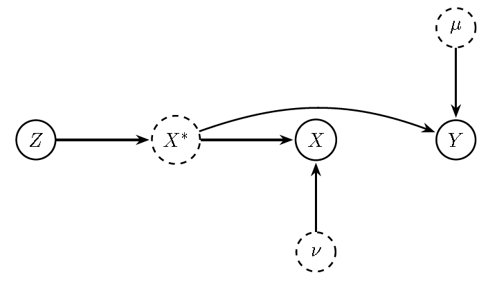
Figure 13.13: DAG with measurement error and instrument \(Z\). Observed \(X\) depends on the latent \(X^{*}\) and error \(v\). Because the composed error in the estimated equation includes \(v\), \(X\) is endogenous when regressed on \(Y\). Instrument \(Z\) isolates exogenous variation in \(X^{*}\).
We simulate the latent process \(X_i^* = 0.5Z_i + e_i\), with the observed regressor defined as \(X_i = X_i^* + \nu_i\), and the outcome equation specified as \(Y_i = 1 + 1.2X_i^* + \mu_i\). The variables \(Z_i\), \(e_i\), and \(\nu_i\) are standard normal, while \(\mu_i\) follows a mixture of two normal distributions with means \(0.5\) and \(-0.5\), and standard deviations \(0.5\) and \(1.2\). The sample size is 2,000, the burn-in is 1,000, and the number of MCMC draws retained after burn-in is 10,000.
We perform Bayesian exponentially tilted empirical likelihood (BETEL) using the package betel, and adopt the default hyperparameter values provided there.77 This package implements Bayesian estimation and marginal likelihood computation for moment condition models, employing a Student-t prior distribution and a Student-t proposal distribution following Siddhartha Chib, Shin, and Simoni (2018). We also compare the results with a model that assumes \(X_i\) is exogenous, and with an instrumental Gibbs sampler that assumes \(Y_i\) is normally distributed. We also use the default hyperparameters of the packages employed. The following code shows the implementation.
The figure displays the posterior distributions. We see that ignoring measurement error produces a biased posterior distribution. In particular, the absolute value of the causal effect is smaller than the population value; this is called attenuation bias. By contrast, methods that account for measurement error and use valid instruments yield well-centered posterior distributions.
## Loading required package: devtools## Loading required package: usethis##
## Attaching package: 'betel'## The following object is masked from 'package:Boom':
##
## rmvn## The following object is masked from 'package:mvtnorm':
##
## rmvt## The following objects are masked from 'package:LaplacesDemon':
##
## rmvn, rmvt, rst## The following object is masked from 'package:MCMCpack':
##
## xpnd## The following object is masked from 'package:sirt':
##
## rmvn# Simulate data
N <- 2000; d <- 2; k <- 2
gamma <- 0.5; beta <- c(1, 1.2)
# Mixture
mum1 <- 1/2; mum2 <- -1/2
mu1 <- rnorm(N, mum1, 0.5); mu2 <- rnorm(N, mum2, 1.2)
mu <- sapply(1:N, function(i){sample(c(mu1[i], mu2[i]), 1, prob = c(0.5, 0.5))})
e <- rnorm(N)
z <- rnorm(N) # Instrument
xlat <- gamma*z + e # Unobserved regressor
nu <- rnorm(N) # Measurement error
x <- xlat + nu # Observed regressor
Xlat <- cbind(1, xlat)
y <- Xlat%*%beta + mu
dat <- cbind(1, x, z) # Data
# Function g_i by row in BETEL
gfunc <- function(psi = psi, y = y, dat = dat) {
X <- dat[,1:2]
e <- y - X %*% psi
E <- e %*% rep(1,d)
Z <- dat[,c(1,3)]
G <- E * Z;
return(G)
}
nt <- round(N * 0.1, 0); # training sample size for prior
psi0 <- lm(y[1:nt]~x[1:nt])$coefficients # Starting value of psi = (theta, v), v is the slack parameter in CSS (2018)
names(psi0) <- c("alpha","beta")
psi0_ <- as.matrix(psi0) # Prior mean of psi
Psi0_ <- 5*rep(1,k) # Prior dispersions of psi
lam0 <- .5*rnorm(d) # Starting value of lambda
nu <- 2.5 # df of the prior student-t
nuprop <- 15 # df of the student-t proposal
n0 <- 1000 # burn-in
m <- 10000 # iterations beyond burn-in
# MCMC ESTIMATION BY THE CSS (2018) method
psim <- betel::bayesetel(gfunc = gfunc, y = y[-(1:nt)], dat = dat[-(1:nt),], psi0 = psi0, lam0 = lam0, psi0_ = psi0_, Psi0_ = Psi0_, nu = nu, nuprop = nuprop, controlpsi = list(maxiterpsi = 50, mingrpsi = 1.0e-8), # list of parameters in maximizing likelihood over psi
controllam = list(maxiterlam = 50, # list of parameters in minimizing dual over lambda
mingrlam = 1.0e-7), n0 = n0, m = m,printstep = 5000)## this is psi0 1.022954 0.6541617
## tailoring to find the proposal has started ...
## $muprop
## alpha beta
## 1.026519 1.284899
##
## $Pprop
## [,1] [,2]
## [1,] 671.68877 14.90052
## [2,] 14.90052 135.87597
##
## $value
## [1] 13497.24
##
## $grad
## [1] -3.375095e-04 -7.844614e-05
##
## this is g 5000
## this is psi1 0.9620988 1.23116
## this is counter/g 0.8704
## this is g 10000
## this is psi1 1.082801 1.311398
## this is counter/g 0.8734
## this is g in numerator of C-J 5000
## this is g in numerator of C-J 10000
## this is g in denominator of C-J 5000
## this is g in denominator of C-J 10000MCMCexg <- MCMCpack::MCMCregress(y ~ x, burnin = n0, mcmc = m)
Data <- list(y = c(y), x = x, z = matrix(z, N, 1), w = matrix(rep(1, N), N, 1))
Mcmc <- list(R = m, nprint = 0)
MCMCivr <- bayesm::rivGibbs(Data, Mcmc = Mcmc)##
## Starting Gibbs Sampler for Linear IV Model
##
## nobs= 2000 ; 1 instruments; 1 included exog vars
## Note: the numbers above include intercepts if in z or w
##
## Prior Parms:
## mean of delta
## [1] 0
## Adelta
## [,1]
## [1,] 0.01
## mean of beta/gamma
## [1] 0 0
## Abeta/gamma
## [,1] [,2]
## [1,] 0.01 0.00
## [2,] 0.00 0.01
## Sigma Prior Parms
## nu= 3 V=
## [,1] [,2]
## [1,] 1 0
## [2,] 0 1
##
## MCMC parms:
## R= 10000 keep= 1 nprint= 0
## dfplot <- data.frame(betel = psim[,2], iv = MCMCivr[["betadraw"]], exo = MCMCexg[,2])
colnames(dfplot) <- c("betel", "iv", "exo")
library(tidyr)
library(dplyr)
library(ggplot2)
df_long <- dfplot |>
pivot_longer(everything(), names_to = "Method", values_to = "Posterior") |>
mutate(Method = factor(Method,
levels = c("betel","iv","exo"),
labels = c("betel","rivGibbs","MCMCregress")))
ggplot(df_long, aes(x = Posterior, color = Method, fill = Method)) +
geom_density(alpha = 0.3, linewidth = 1) +
geom_vline(xintercept = 1.2, linetype = "dashed", linewidth = 1, color = "black") +
labs(
title = "Posterior Densities with Population Value",
x = expression(beta[1]),
y = "Density"
) +
theme_minimal(base_size = 14) +
theme(
legend.position = "top",
legend.title = element_blank()
)
Example: Omission of relevant correlated regressor
Consider the true model
\[ Y_i = \beta_0 + \beta_1 X_i + \gamma W_i + \mu_i, \qquad \mathbb{E}[\mu_i \mid X_i, W_i] = 0. \]
Suppose that the relevant regressor \(W_i\) is omitted from the specification, with \(\gamma \neq 0\) and \(\operatorname{Cov}(X_i, W_i) \neq 0\).
Thus, if we regress \(Y_i\) only on \(X_i\), the composite error is
\[ \epsilon_i = \gamma W_i + \mu_i. \]
Therefore,
\[ \mathbb{E}[\epsilon_i \mid X_i] = \gamma \, \mathbb{E}[W_i \mid X_i] + \mathbb{E}[\mu_i \mid X_i] = \gamma \, \mathbb{E}[W_i \mid X_i] \neq 0, \]
since \(\mathbb{E}[W_i \mid X_i]\) is nonconstant whenever \(X_i\) and \(W_i\) are correlated, that is, the expected value of \(W_i\) is a function of \(X_i\).
Consequently,
\[ \mathbb{E}[\epsilon_i X_i] = \gamma \, \mathbb{E}[W_i X_i] + \mathbb{E}[\mu_i X_i]. \]
Because \(\mathbb{E}[\mu_i X_i]=0\), we obtain
\[ \mathbb{E}[\epsilon_i X_i] = \gamma (\operatorname{Cov}(W_i,X_i) + \mathbb{E}[W_i] \, \mathbb{E}[X_i])\neq 0. \]
In this situation, we can use an instrument that is relevant (\(\mathbb{E}[Z_i X_i] \neq 0\)) and exogenous (\(\mathbb{E}[Z_i \mid \mu_i] = \mathbb{E}[Z_i \mid W_i] = 0\)) to address the endogeneity problem, and identify the causal effect.78 Therefore,
\[ \mathbb{E}\left[\begin{bmatrix} 1\\ Z_i \end{bmatrix}(Y_i-\beta_0-\beta_1X_i)\right]=\mathbf{0}. \]
The figure illustrates the case of an omitted relevant regressor that is correlated with \(X_i\), and how an instrument can be used to identify the causal effect. The instrument resolves the endogeneity problem by exploiting variation in \(X_i\) that is driven by \(Z_i\), which is orthogonal to the problematic error term. In other words, it replaces “bad” correlation with “clean” variation.
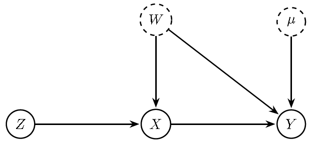
Figure 13.14: DAG with omitted relevant regressor \(W\) (dashed, unobserved) that is correlated with \(X\) and affects \(Y\), inducing endogeneity of \(X\) in a regression of \(Y\) on \(X\). A valid instrument \(Z\) affects \(X\) (relevance) but has no direct path to \(Y\) and is independent of \(W\) and \(u\) (exclusion/independence), enabling identification of the causal effect \(X\) on \(Y\).
We ask in Exercise 10 to perform a simulation exercise to assess the ability of BETEL to identify the causal effect when an instrument is used to address the omission of relevant regressors.
Example: Simultaneous causality
This example is based on Guido W. Imbens (2014), where Professor Imbens illustrates the problem of analyzing the causal effect on traded quantity of a tax of \(100 \times r\%\) in a market. He defines the average causal effect on the logarithm of traded quantity is
\[ \tau = \mathbb{E}[q_i(r) - q_i(0)], \]
where \(q_i(r) = \log Q_i(r)\) and \(Q_i(r)\) denotes the potential traded quantity if the tax were \(r\)%.
This situation is more challenging than in the standard treatment effects literature, because we do not observe any unit facing the tax. Instead, we only observe all units facing no tax, that is, \(Q_i^{\text{Obs}} = Q_i(0)\). This setting requires the use of a structural model to define the counterfactual scenarios of the potential outcomes.
The starting point for inference on the treatment effect of this new tax is the price determination mechanism, that is, the assignment mechanism in the potential outcome framework. We specify a structural demand function that defines the potential demand given the price (treatment) and other exogenous variables:
\[ q_i^d(p) = \beta_1 + \beta_2 p + \beta_3 y_i + \beta_4 pc_i + \beta_5 ps_i + u_{i1}, \]
where \(q^d\) is demand, and \(p\), \(y\), \(pc\), and \(ps\) are the logarithms of price, income, the price of a complementary good, and the price of a substitute good, respectively. All coefficients are interpreted as demand elasticities. The term \(u_{i1}\) represents unobserved demand factors such that \(\mathbb{E}[u_{i1}]=0\). Therefore,
\[ \mathbb{E}[q_i^d(p)\mid p, y_i, pc_i, ps_i] = \beta_1 + \beta_2 p + \beta_3 y_i + \beta_4 pc_i + \beta_5 ps_i. \]
This expectation does not represent the conditional expectation of the observed quantity in markets where the observed price equals \(p\). Rather, it is the expectation of potential demand functions given \(p\) and other exogenous controls, irrespective of the realized market price.
Similarly, the assignment mechanism requires specifying the structural supply function:
\[ q_i^s(p) = \alpha_1 + \alpha_2 p + \alpha_3 er_i + u_{i2}, \]
which represents the quantity that sellers are willing to supply given the price and the (exogenous) exchange rate \(er_i\). The unobserved supply factors satisfy \(\mathbb{E}[u_{i2}]=0\), so that
\[ \mathbb{E}[q_i^s(p)\mid p, er_i] = \alpha_1 + \alpha_2 p + \alpha_3 er_i. \]
This expectation represents the average of all potential supply functions given the price and exogenous controls, again irrespective of the realized market price.
Thus, the assignment mechanism is given by the market equilibrium where the observed price is such that the observed quantity is equal to the demand and supply potential outcomes at the observed price,
\[ q_i^{Obs}=q_i^d(p_i^{Obs})=q_i^s(p_i^{Obs}). \]
Using this market equilibrium condition, we get
\[ p_i^{Obs}=\pi_1+\pi_2 er_i + \pi_3 y_i + \pi_4 pc_i + \pi_5 ps_i + v_{i1}, \]
where \(\pi_1=\frac{\alpha_1-\beta_1}{\beta_2-\alpha_2}\), \(\pi_2=\frac{\alpha_3}{\beta_2-\alpha_2}\), \(\pi_3=\frac{-\beta_3}{\beta_2-\alpha_2}\), \(\pi_4=\frac{-\beta_4}{\beta_2-\alpha_2}\), \(\pi_5=\frac{-\beta_5}{\beta_2-\alpha_2}\), and \(v_{i1}=\frac{u_{i2}-u_{i1}}{\beta_2-\alpha_2}\) given \(\beta_2\neq\alpha_2\), that is, the equations should be independent. This condition is given by economic theory due to \(\beta_2<0\) and \(\alpha_2>0\), the effect of price on demand and supply should be negative and positive, respectively.
The equation of price into the demand equation gives
\[ q_i^{Obs}=\tau_1+\tau_2 er_i + \tau_3 y_i + \tau_4 pc_i + \tau_5 ps_i + v_{i2}, \]
where \(\tau_1=\beta_1+\beta_2\pi_1\), \(\tau_2=\beta_2\pi_2\), \(\tau_3=\beta_2\pi_3+\beta_3\), \(\tau_4=\beta_2\pi_4+\beta_4\), \(\tau_5=\beta_2\pi_5+\beta_5\), and \(v_{i2}=\beta_2v_{i1}+u_{i1}\).
The expressions for \(p_i^{Obs}\) and \(q_i^{Obs}\) are called the reduced-form representations. In Section 7.1, we presented the order condition, which is necessary, and the rank condition, which is both necessary and sufficient, to identify the structural parameters from the reduced-form parameters. A key point to note is that only the prior distribution of the reduced-form parameters is updated by the sample information, while the updating of the structural parameters occurs solely through the reduced-form parameters, that is,
\[ \pi(\boldsymbol{\beta},\boldsymbol{\alpha}\mid \boldsymbol{\gamma},\boldsymbol{\pi},\mathbf{W}_{1:N}) \;\propto\; \pi(\boldsymbol{\beta},\boldsymbol{\alpha}\mid \boldsymbol{\gamma},\boldsymbol{\pi}). \]
See Section 9.3 in Zellner (1996b) for details about identification in Bayesian inference. This implies that in under-identified models, the posterior distribution of the structural parameters is not concentrated at a single point, but rather remains spread out (e.g., uniformly) over a range of values.79
To analyze the causal effects of the new tax, we can find the new equilibrium,
\[ q_i^d(P_i(r)\times (1+r))=q_i^s(P_i(r)), \]
where \(P_i(r)\) is the price level (\(p_i(r)=\log P_i(r)\)) that sellers get, and \((P_i(r)\times (1+r)\) is the price that buyers pay.
Let’s define the (log) price that buyers pay \(p_b = p + \log(1+r)\) while sellers receive \(p\). The demand function becomes
\[ q_i^d\big(p + \log(1+r)\big) = \beta_1 + \beta_2\left(p + \log(1+r)\right) + \beta_3 y_i + \beta_4 pc_i + \beta_5 ps_i + u_{i1}, \]
and the supply function remains
\[ q_i^s(p) = \alpha_1 + \alpha_2 p + \alpha_3 er_i + u_{i2}. \]
Thus, the equilibrium price is given by
\[ p_i^*(r) = \frac{(\beta_1 - \alpha_1) + \beta_3 y_i + \beta_4 pc_i + \beta_5 ps_i - \alpha_3 er_i + (u_{i1} - u_{i2}) + \beta_2 \log(1+r)}{\alpha_2 - \beta_2}. \]
The equilibrium quantity is
\[ q_i^*(r) = \beta_1 + \beta_2\left(p_i^*(r) + \log(1+r)\right) + \beta_3 y_i + \beta_4 pc_i + \beta_5 ps_i + u_{i1}. \]
Thus, the expected equilibrium price and quantity are
\[ \mathbb{E}[p_i^*(r)\mid y_i, pc_i, ps_i, er_i] = \frac{(\beta_1 - \alpha_1) + \beta_3 y_i + \beta_4 pc_i + \beta_5 ps_i - \alpha_3 er_i + \beta_2 \log(1+r)}{\alpha_2 - \beta_2}, \]
\[ \mathbb{E}[q_i^*(r)\mid y_i, pc_i, ps_i, er_i] = \alpha_1 + \alpha_2 \,\mathbb{E}[p_i^*(r)\mid \cdot] + \alpha_3 er_i. \]
We can see that given \(\beta_2 < 0 < \alpha_2\), we have:
\[ \frac{d p^*(r)}{dr} = \frac{\beta_2}{(\alpha_2 - \beta_2)(1+r)} < 0, \quad \frac{d p_b^*(r)}{dr} = \frac{\alpha_2}{(\alpha_2 - \beta_2)(1+r)} > 0, \quad \frac{d q^*(r)}{dr} = \alpha_2 \cdot \frac{d p^*(r)}{dr} < 0. \]
Thus, the price received by sellers decreases with the tax, the price paid by buyers increases, and the equilibrium quantity falls.
Thus, the average causal effect on the logarithm of traded quantity is
\[ \tau = \mathbb{E}[q_i(r) - q_i(0)]= \frac{\alpha_2 \, \beta_2}{\alpha_2 - \beta_2}\,\log(1+r). \]
Note that the treatment effect depends on the price elasticities of supply and demand. Therefore, we need to identify the demand and supply functions using instruments, since the observed quantities and prices cannot be used directly due to the issue of simultaneous causality. In particular, given the assumption of exogeneity of the other control variables, the only part of \(p_i^{Obs}\) that can correlate with \(u_{i1}\) or \(u_{i2}\) is the error component
\[ \frac{u_{i2}-u_{i1}}{\beta_2-\alpha_2}. \]
Hence
\[ \mathbb{E}[u_{i1}p_i^{Obs}] =\frac{1}{\beta_2-\alpha_2}\,\mathbb{E}\!\big[u_{i1}(u_{i2}-u_{i1})\big] =\frac{\operatorname{Cov}(u_{i1},u_{i2})-\operatorname{Var}(u_{i1})}{\beta_2-\alpha_2}\neq 0, \]
and
\[ \mathbb{E}[u_{i2}p_i^{Obs}] =\frac{1}{\beta_2-\alpha_2}\,\mathbb{E}\!\big[u_{i2}(u_{i2}-u_{i1})\big] =\frac{\operatorname{Var}(u_{i2})-\operatorname{Cov}(u_{i1},u_{i2})}{\beta_2-\alpha_2}\neq 0, \]
due to the usual slopes \(\beta_2<0<\alpha_2\) so that \(\alpha_2-\beta_2>0\).
We can use supply shifters to identify the demand, and demand shifters to identify the supply. In this setting, the exchange rate serves as an instrument to identify the demand, while income together with the prices of complementary and substitute goods serve as instruments to identify the supply. Thus, we can use the moment conditions,
\[ \mathbb{E}\left[\begin{bmatrix} 1\\ y_i\\ pc_i\\ ps_i\\ er_i \end{bmatrix}(q_i^{Obs}-\beta_1-\beta_2p_i^{Obs}-\beta_3y_i-\beta_4pc_i-\beta_5ps_i)\right]=\mathbf{0}, \]
and
\[ \mathbb{E}\left[\begin{bmatrix} 1\\ y_i\\ pc_i\\ ps_i\\ er_i \end{bmatrix}(q_i^{Obs}-\alpha_1-\alpha_2p_i^{Obs}-\alpha_3er_i)\right]=\mathbf{0} \]
to identify the demand and supply functions. Note that the demand equation is exactly identified, whereas the supply equation is over-identified.
We perform a simulation exercise to analyze the hypothetical causal effects of a new tax rate of 10% simulating the demand and supply equations using the following structural parameters \(\boldsymbol{\beta} = \left[ 5 \ -0.5 \ 0.8 \ -0.4 \ 0.7 \right]^{\top}\), \(\boldsymbol{\alpha} = \left[ -2 \ 0.5 \ -0.4 \right]^{\top}\), \(u_1 \sim N(0, 0.5^2)\), and \(u_2 \sim N(0, 0.5^2)\) assuming a sample size equal to 5,000. Additionally, assume that \(y \sim N(10, 1)\), \(pc \sim N(5, 1)\), \(ps \sim N(5, 1)\), and \(er \sim N(15, 1)\).
The population causal effect of the tax on quantity is
\[ \tau=\frac{(-0.5)\times 0.5}{0.5-(-0.5)}\log(1+0.1)\approx -0.0238, \]
which implies that a 10% tax reduces traded quantity by approximately 2.4%.
In Exercise 11, you are asked to program a BETEL algorithm from scratch to perform inference in this example. Th following figure displays the posterior distribution of the causal effect. The 95% credible interval contains the population value, and the posterior mean lies close to it.
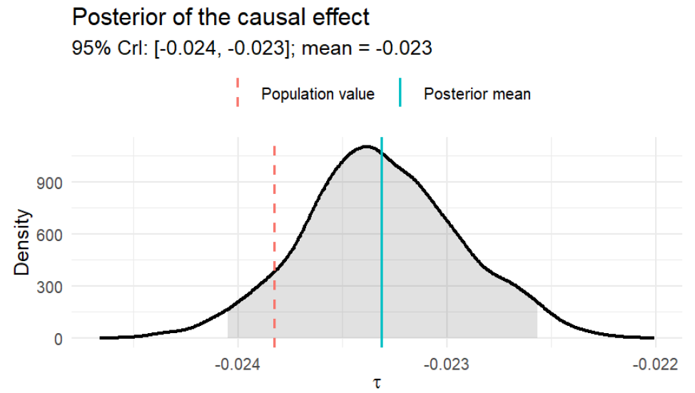
Figure 13.15: Posterior distribution of the causal effect of a tax: BETEL
Siddhartha Chib, Shin, and Simoni (2018) propose a unified framework based on marginal likelihoods and Bayes factors for comparing different moment-restricted models and for discarding misspecified restrictions. They demonstrate the model selection consistency of the marginal likelihood, showing that it favors the specification with the fewest parameters and the largest number of valid moment restrictions. When models are misspecified, the marginal likelihood procedure selects the model that is closest to the (unknown) true data-generating process in terms of Kullback–Leibler divergence. See Nicole A. Lazar (2021) and P. Liu and Zhao (2023) for comprehensive reviews of recent advances in empirical likelihood and exponentially tilted empirical likelihood methods, including their Bayesian variants.
References
Available at https://apps.olin.wustl.edu/faculty/chib/rpackages/betel/.↩︎
Another potential solution for the omission of relevant variables is the use of proxy variables; see Jeffrey M. Wooldridge (2010) for details.↩︎
This identification issue is not peculiar to simultaneous equation models, it arises in other econometric/statistical models (Zellner 1996b). See for instance the example of the effects of vitamin A.↩︎