6.9 Interactions
Just like with linear regression, you can include an interaction in a logistic regression model to evaluate if a predictor is an effect modifier, that is, if the OR for one predictor depends on another (the effect modifier).
Example 6.3 (continued): After adjusting for age and income, does the association between lifetime marijuana use and age at first use of alcohol differ by sex?
Adding the interaction term alc_agefirst:demog_sex to the model, we get the following results.
fit.ex6.3.int <- glm(mj_lifetime ~ alc_agefirst + demog_age_cat6 + demog_sex +
                     demog_income + alc_agefirst:demog_sex,
           family = binomial, data = nsduh)
round(summary(fit.ex6.3.int)$coef, 4)
## Estimate Std. Error z value Pr(>|z|)
## (Intercept) 7.3735 0.8292 8.8923 0.0000
## alc_agefirst -0.3378 0.0423 -7.9876 0.0000
## demog_age_cat626-34 -0.2951 0.3314 -0.8902 0.3733
## demog_age_cat635-49 -0.8160 0.2987 -2.7320 0.0063
## demog_age_cat650-64 -0.6866 0.3007 -2.2832 0.0224
## demog_age_cat665+ -1.2600 0.3064 -4.1130 0.0000
## demog_sexMale -2.1381 0.9847 -2.1713 0.0299
## demog_income$20,000 - $49,999 -0.5304 0.2682 -1.9773 0.0480
## demog_income$50,000 - $74,999 -0.0931 0.3073 -0.3029 0.7620
## demog_income$75,000 or more -0.3629 0.2547 -1.4250 0.1542
## alc_agefirst:demog_sexMale 0.1189 0.0555 2.1420 0.0322To answer the question of significance, look at the row in the regression coefficients table corresponding to the interaction (alc_agefirst:demog_sex). The p-value is 0.0322, so the interaction is statistically significant. Had there been more than one row (e.g., if the interaction involved a categorical predictor with more than two levels), then use a Type III test to get the test of interaction. Since, in this case, there is just one term corresponding to the interaction, the Type III Wald test p-value from car::Anova() is exactly the same as the p-value in the coefficients table.
## Analysis of Deviance Table (Type III tests)
##
## Response: mj_lifetime
##                        Df Chisq           Pr(>Chisq)
## (Intercept)             1 79.07 < 0.0000000000000002 ***
## alc_agefirst            1 63.80   0.0000000000000014 ***
## demog_age_cat6          4 22.33              0.00017 ***
## demog_sex               1  4.71              0.02991 *
## demog_income            3  5.23              0.15555
## alc_agefirst:demog_sex  1  4.59              0.03219 *
## ---
## Signif. codes:  0 '***' 0.001 '**' 0.01 '*' 0.05 '.' 0.1 ' ' 1
Conclusion: The association between age of first alcohol use and lifetime marijuana use differs significantly between males and females (p = .032).
6.9.1 Overall test of a predictor involved in an interaction
As shown in Section 5.10.11 for MLR, to carry out an overall test of a predictor involved in an interaction in a regression model, compare the full model to a reduced model with both the main effect and interaction removed. As with MLR, use anova() to compare the models, but for a logistic regression you must also specify test = "Chisq" to get a p-value. If you did not remove missing data prior to fitting the full model, you must do so before comparing models if the main effect predictor being removed to create the reduced model has missing values. You can either create a new dataset with missing values removed or use the subset option.
Example 6.3 (continued): In the model that includes an interaction, is age at first alcohol use significantly associated with the outcome?
# Fit the reduced model using the subset option
# to remove missing values for the predictor
# being removed to create the reduced model
fit0 <- glm(mj_lifetime ~ demog_age_cat6 + demog_sex + demog_income,
           family = binomial, data = nsduh,
           subset = complete.cases(alc_agefirst))
# Compare to full model
anova(fit0, fit.ex6.3.int, test = "Chisq")
## Analysis of Deviance Table
##
## Model 1: mj_lifetime ~ demog_age_cat6 + demog_sex + demog_income
## Model 2: mj_lifetime ~ alc_agefirst + demog_age_cat6 + demog_sex + demog_income +
## alc_agefirst:demog_sex
## Resid. Df Resid. Dev Df Deviance Pr(>Chi)
## 1 834 1085
## 2 832 931 2 154 <0.0000000000000002 ***
## ---
## Signif. codes: 0 '***' 0.001 '**' 0.01 '*' 0.05 '.' 0.1 ' ' 1The 2 df test (2 df because the models differ in two terms – the main effect and the interaction) results in a very small p-value.
Conclusion: Age at first alcohol use is significantly associated with the outcome (p <.001).
6.9.2 Estimate the OR at each level of the other predictor
Use gmodels::estimable() to compute separate ORs for a predictor involved in an interaction at each level of the other predictor in the interaction. When there is no interaction, or when there is one but the other predictor in the interaction is zero or at its reference level, the OR for a predictor is its exponentiated regression coefficient. When there is an interaction and the other predictor is non-zero or at a non-reference level, add the appropriate interaction term multiplied by the value of the other predictor to the main effect before exponentiating. Do not add the intercept or any other terms in the model since when computing the odds ratio all other terms drop out of the equation. In particular, do not add the main effect coefficient for the other predictor in the interaction.
Example 6.3 (continued): In the model that includes an interaction, what are the AORs for age at first alcohol use for females and males?
Before using gmodels::estimable(), look at the coefficient names in the glm object to make sure you spell them correctly.
##  [1] "(Intercept)"                   "alc_agefirst"
##  [3] "demog_age_cat626-34"           "demog_age_cat635-49"
##  [5] "demog_age_cat650-64"           "demog_age_cat665+"
##  [7] "demog_sexMale"                 "demog_income$20,000 - $49,999"
##  [9] "demog_income$50,000 - $74,999" "demog_income$75,000 or more"
## [11] "alc_agefirst:demog_sexMale"
# ORs for alc_agefirst
# Other predictor in the interaction is sex
# Females (reference level of other predictor)
EST.F <- gmodels::estimable(fit.ex6.3.int,
c("alc_agefirst" = 1),
conf.int = 0.95)
# Males (non-reference level of other predictor)
EST.M <- gmodels::estimable(fit.ex6.3.int,
c("alc_agefirst" = 1,
"alc_agefirst:demog_sexMale" = 1),
conf.int = 0.95)
rbind(EST.F, EST.M)## Estimate Std. Error X^2 value DF Pr(>|X^2|)
## (0 1 0 0 0 0 0 0 0 0 0) -0.3378 0.04229 63.80 1 0.000000000000001332
## (0 1 0 0 0 0 0 0 0 0 1) -0.2189 0.03626 36.43 1 0.000000001581411446
## Lower.CI Upper.CI
## (0 1 0 0 0 0 0 0 0 0 0) -0.4217 -0.2539
## (0 1 0 0 0 0 0 0 0 0 1) -0.2908 -0.1469These estimates are on the log-odds-ratio scale. We need to exponentiate to get AORs. But we have to be careful because the gmodels::estimable() output includes a p-value, and we do not want to exponentiate that. The code below exponentiates just the estimate and 95% CI.
# AORs and 95% CIs (do use exp here)
rbind(exp(EST.M[c("Estimate", "Lower.CI", "Upper.CI")]),
      exp(EST.F[c("Estimate", "Lower.CI", "Upper.CI")]))
## Estimate Lower.CI Upper.CI
## (0 1 0 0 0 0 0 0 0 0 1) 0.8034 0.7476 0.8633
## (0 1 0 0 0 0 0 0 0 0 0) 0.7133 0.6559 0.7758## Pr(>|X^2|)
## (0 1 0 0 0 0 0 0 0 0 1) 0.000000001581411446
## (0 1 0 0 0 0 0 0 0 0 0) 0.000000000000001332Conclusion: After adjusting for age and income, age at first alcohol use is significantly associated with lifetime marijuana use (p <.001 – from the test comparing the model with an interaction to the model with no alc_agefirst main effect or interaction). The association between age at first alcohol use and lifetime marijuana use differs significantly between males and females (interaction p = .032). An age of first alcohol use 1 year greater is associated with 19.7% lower odds of lifetime marijuana use for males (AOR = 0.803; 95% CI = 0.748, 0.863; p <.001) and 28.7% lower odds for females (AOR = 0.713; 95% CI = 0.656, 0.776; p <.001).
NOTE: The above example was for a continuous \(\times\) categorical interaction. For a categorical \(\times\) categorical or continuous \(\times\) continuous interaction, imitate the code in Section 5.10.9.2 or 5.10.9.3, respectively, and then exponentiate the resulting estimates and CIs (but do not exponentiate the p-values).
6.9.3 Visualize an interaction
It is always a good idea to visualize the magnitude of an interaction effect. Remember, in a large sample an effect can be statistically significant without being meaningfully large (practically significant) and, in a small sample, an effect can lack statistical significance but still be meaningfully large. Visualizing the effect can help with assessing practical significance.
Example 6.3 (continued): Visualize the interaction between age of first alcohol use and sex. The code below produces Figure 6.4.
We use plot_model() as we did with multiple linear regression. Note the addition of [all] after alc_agefirst which specifies plotting at all the possible values of the variable. Typically, [all] is not needed, but leaving it out in this example results in a curve that does not look smooth.
library(sjPlot)

# Effect of alc_agefirst at each level of demog_sex
plot_model(fit.ex6.3.int,
           type = "eff",
           terms = c("alc_agefirst [all]", "demog_sex"),
           title = "",
           axis.title = c("Age of First Alcohol Use (years)",
                          "P(Lifetime Marijuana Use)"),
           legend.title = "Sex")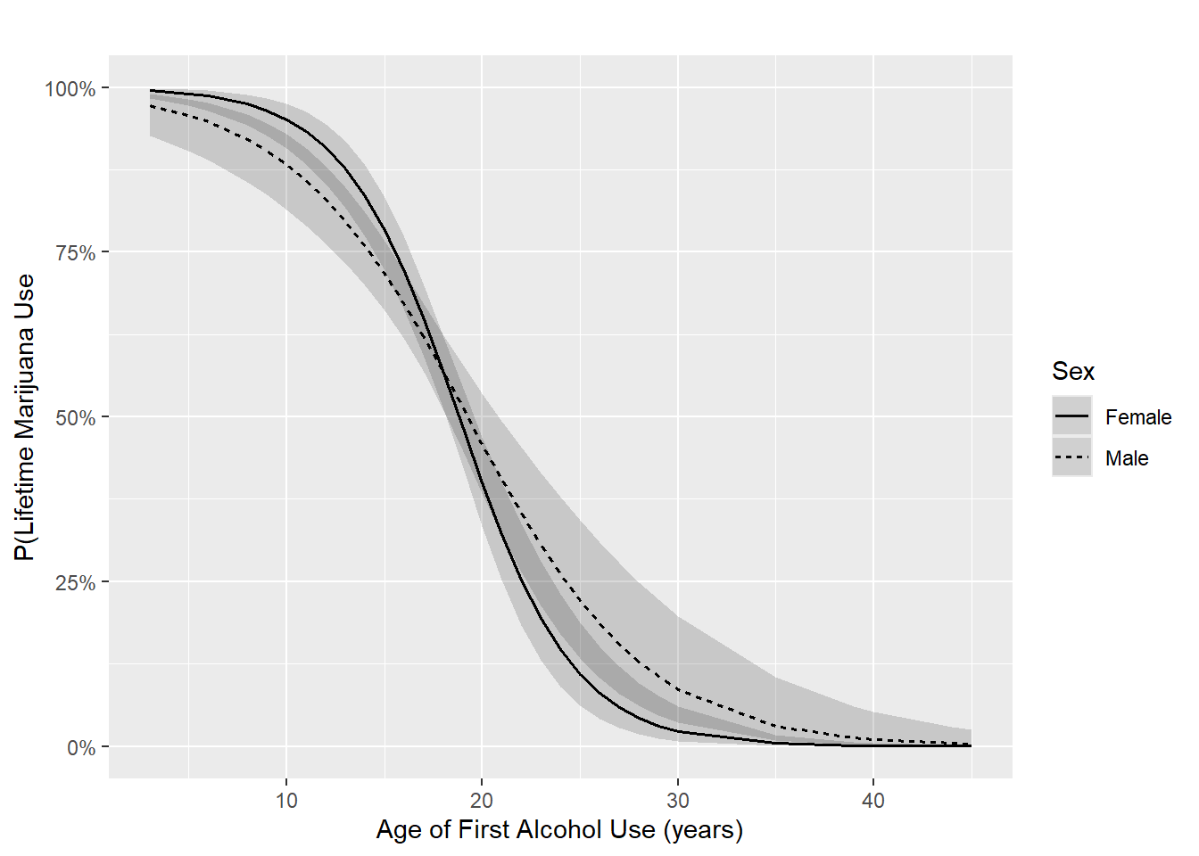
Figure 6.4: Logistic regression interaction plot
Conclusion: We previously concluded that the interaction was statistically significant. In linear regression, this is equivalent to concluding that the fitted lines are significantly different from parallel. The same is true for logistic regression, but only on the log-odds scale. On the probability scale, as shown in Figure 6.4, we have fitted curves, not lines. However, the shape of the curves do appear to be meaningfully different from each other, indicating that the magnitude of the interaction is meaningfully large.