5.16 Checking the normality assumption
Earlier in this chapter we stated that \(\epsilon \sim N(0, \sigma^2)\) which is, in part, shorthand for “the errors are normally distributed around the mean outcome and the average of the errors is zero”. This implies that at any given predictor value the distribution of \(Y\) given \(X\) is assumed to be normal. For example, in Figure 5.20, the SLR on the left meets the normality assumption, while the one on the right (from Example 4.1) does not.
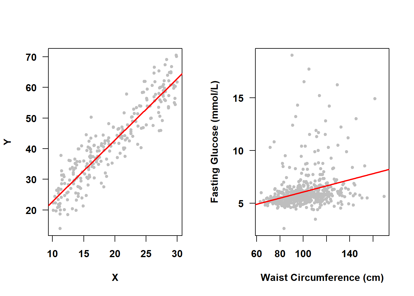
Figure 5.20: Normality assumption met vs. not met
5.16.1 Impact of non-normality
A violation of the assumption of normality of errors may result in incorrect inferences in small samples. Both confidence intervals and p-values rely on the normality assumption, so if it is not valid then these may be inaccurate. However, in large samples (at least ten observations per predictor, although this is just a rule of thumb (Schmidt and Finan 2018)) violation of the normality assumption does not have much of an impact on inferences (Weisberg 2014).
5.16.2 Diagnosis of non-normality
The assumption is that the errors are normally distributed. We do not actually observe the errors, but we do observe the residuals and so we use those to diagnose normality (as well as other assumptions). There are formal tests of normality (e.g., the Shapiro-Wilk test); however, they are not needed in large samples since violation of the normality assumption will not impact inferences and they lack power in small samples. Instead, use a visual diagnosis.
While Figure 5.20 provided a general illustration, two diagnostic tools that allow us to directly compare the residuals to a normal distribution are a histogram of the residuals and a normal quantile-quantile plot (QQ plot), both of which are explained in the following example.
To illustrate the diagnosis of non-normality in a small sample size, we will use a random subset of 50 observations from our NHANES fasting subsample dataset (nhanesf.complete.50_rmph.Rdata) and re-fit the model from Example 5.1.
Example 5.1 (continued): Diagnose non-normality in the small sample size version of Example 5.1. Plot the residuals using a histogram and QQ plot.
load("Data/nhanesf.complete.50_rmph.Rdata")

# Re-fit the model using the small n dataset
fit.ex5.1.smalln <- lm(LBDGLUSI ~ BMXWAIST + smoker + RIDAGEYR +
                         RIAGENDR + race_eth + income,
                       data = nhanesf.complete.50)

# View results
round(cbind(summary(fit.ex5.1.smalln)$coef,
            confint(fit.ex5.1.smalln)),4)
## Estimate Std. Error t value Pr(>|t|) 2.5 % 97.5 %
## (Intercept) 3.1771 1.5706 2.0228 0.0500 0.0002 6.3540
## BMXWAIST 0.0258 0.0102 2.5390 0.0152 0.0052 0.0464
## smokerPast -0.4796 0.5278 -0.9088 0.3690 -1.5471 0.5879
## smokerCurrent 0.5608 0.6197 0.9048 0.3711 -0.6928 1.8143
## RIDAGEYR 0.0168 0.0139 1.2109 0.2332 -0.0113 0.0448
## RIAGENDRFemale -1.0163 0.4812 -2.1120 0.0411 -1.9896 -0.0430
## race_ethNon-Hispanic White 0.0297 0.6071 0.0489 0.9612 -1.1983 1.2577
## race_ethNon-Hispanic Black 0.2479 0.8903 0.2785 0.7821 -1.5528 2.0487
## race_ethNon-Hispanic Other 2.2347 0.8800 2.5393 0.0152 0.4547 4.0147
## income$25,000 to <$55,000 -0.1413 0.7488 -0.1886 0.8514 -1.6559 1.3734
## income$55,000+ -0.2065 0.6999 -0.2951 0.7695 -1.6223 1.2092# Compute residuals
RESID <- fit.ex5.1.smalln$residuals
# Sample size vs. # of predictors
length(RESID)## [1] 50## [1] 10There are fewer than 10 observations per predictor (50 / 10 = 5).
par(mfrow=c(1,2))
hist(RESID, xlab = "Residuals", probability = T,
     # Adjust ylim to be able to see more of the curves if needed
     ylim = c(0, 0.6))
# Superimpose empirical density (no normality assumption, for comparison)
lines(density(RESID, na.rm=T), lwd = 2, col = "red")
# Superimpose best fitting normal curve
curve(dnorm(x, mean = mean(RESID, na.rm=T), sd = sd(RESID, na.rm=T)),
      lty = 2, lwd = 2, add = TRUE, col = "blue")

# Normal quantile-quantile (QQ) plot
# (use standardized residuals)
qqnorm(rstandard(fit.ex5.1.smalln), col="red", pch=20)
abline(a=0, b=1, col="blue", lty=2, lwd=2)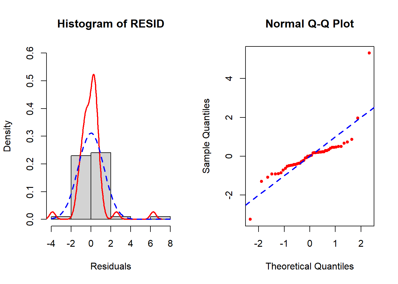
Figure 5.21: Diagnosis of normality of errors
In the left panel (histogram of residuals) of Figure 5.21, the solid line provides a smoothed estimate of the distribution of the observed residuals without making any assumption about the shape of the distribution. The dashed line, however, is the best fit normal curve. The closer these two curves are to each other, the better the normality assumption is met. In the right panel (a QQ plot), the ordered values of the \(n\) residuals are plotted against the corresponding \(n\) quantiles of the standard normal distribution. The closer the points are to the dashed line, the better the normality assumption is met. In this example, there is a lack of normality in the tails of the distribution. Since the sample size is small (n = 50, 10 predictors, fewer than 10 per predictor), non-normality may impact the results.
For convenience, instead of all the code above you can use the check_normality() function found in Functions_rmph.R (which you loaded at the beginning of this chapter).
5.16.3 Potential solutions for non-normality
If the sample size is large (at least ten observations per predictor, although this is just a rule of thumb (Schmidt and Finan 2018)), non-normality does not need to be addressed (Weisberg 2014).
If the sample size is not large: Some alternative methods of handling non-normality include the following.
- Non-normality may co-occur with non-linearity and/or non-constant variance. It is a good idea to check all the assumptions, and then resolve the most glaring assumption failure first, followed by re-checking all the assumptions to see what problems remain. Transforming the outcome is often a good place to start and can help with all three assumptions.
- Normalizing transformation: A transformation of the outcome \(Y\) used to correct non-normality of errors is called a “normalizing transformation”. Common transformations are natural logarithm, square root, and inverse. These are all special cases of the Box-Cox family of outcome transformations which we will discuss in Section 5.19.
- Unfortunately, these transformations only work for positive outcomes. An exception is the square-root transformation which can handle zeros, but still not negative values. For the other transformations, if the outcome is non-negative but includes some zero values, it is common to add 1 before transforming (e.g., \(\log(X+1)\)). If the values of the raw variable are all very small or large, then instead of adding 1, add a number on a different scale (e.g., 0.01, 0.10, 10, 100). However, this approach is arbitrary, and the final results can depend on the number chosen. A sensitivity analysis can be useful to check if the results change when adding a different number (see Section 5.26).
- If the outcome has many zero values, however, then no transformation will result in normality – there will always be a spike in the distribution at that (transformed) value. An alternative is to transform the variable into a binary or ordinal variable and use logistic regression (see Chapter 6), or use a regression method designed for non-negative data such as Poisson regression, zero-inflated Poisson regression, or negative binomial regression (Zeileis, Kleiber, and Jackman 2008).
NOTE: A regression model does not assume that either the outcome or predictors are normally distributed. Rather, it assumes that the errors are normally distributed. It is often the case, however, that the normality or non-normality of the outcome (\(Y\)) does correspond to that of the errors.
Example 5.1 (continued): Continuing with our small sample size version of this example, examine if the natural logarithm, square-root, or inverse normalizing transformations correct the lack of normality.
Figures 5.22 to 5.25 display the histograms and QQ plots of residuals after these three transformations. Since the inverse transformation reverses the ordering of the variable, to preserve the original ordering also multiply by –1.
##    Min. 1st Qu.  Median    Mean 3rd Qu.    Max.
##    4.55    5.27    5.61    5.97    6.11   16.20
# All positive so we can use log, sqrt, or inverse
fit.ex5.1.logY <- lm(log(LBDGLUSI) ~ BMXWAIST + smoker + RIDAGEYR +
RIAGENDR + race_eth + income, data = nhanesf.complete.50)
fit.ex5.1.sqrtY <- lm(sqrt(LBDGLUSI) ~ BMXWAIST + smoker + RIDAGEYR +
RIAGENDR + race_eth + income, data = nhanesf.complete.50)
fit.ex5.1.invY <- lm(-1/LBDGLUSI ~ BMXWAIST + smoker + RIDAGEYR +
RIAGENDR + race_eth + income, data = nhanesf.complete.50)# Histograms and QQ plots of residuals
# sample.size=F suppresses printing of the sample size
check_normality(fit.ex5.1.smalln, sample.size=F, main = "Y")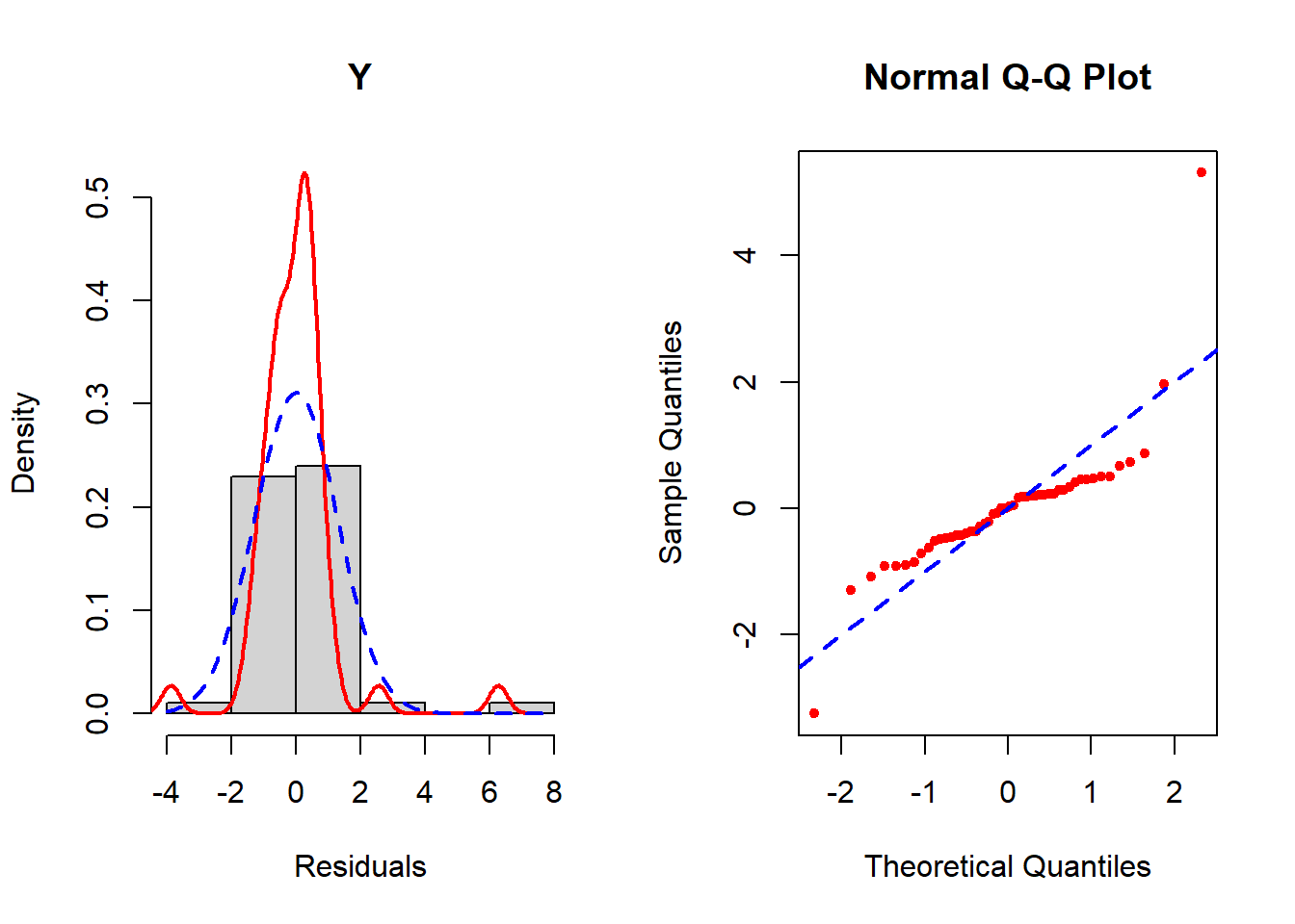
Figure 5.22: Checking the normality assumption (untransformed outcome)
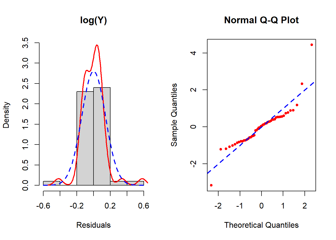
Figure 5.23: Checking the normality assumption (log-transformed outcome)
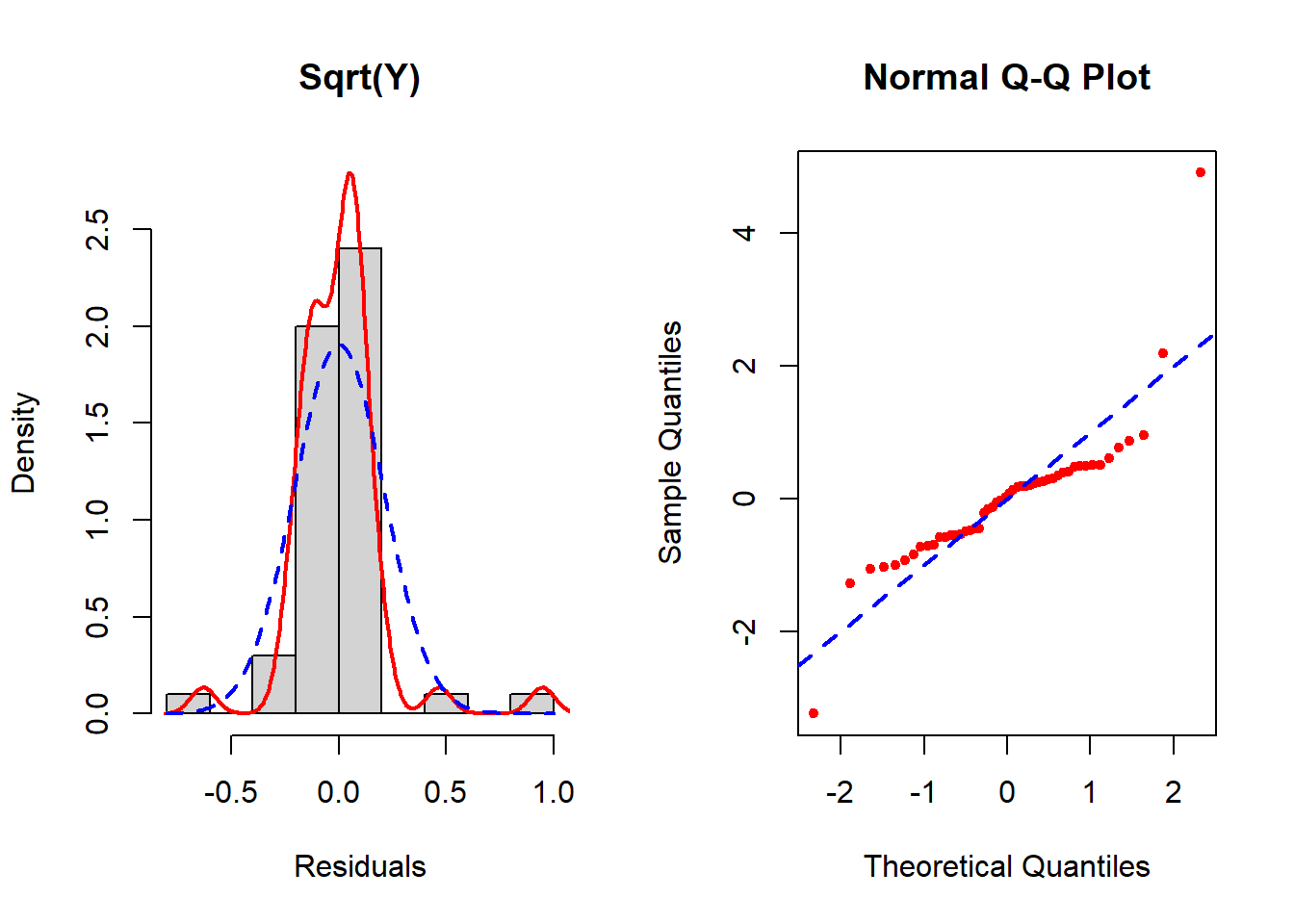
Figure 5.24: Checking the normality assumption (square root transformed outcome)
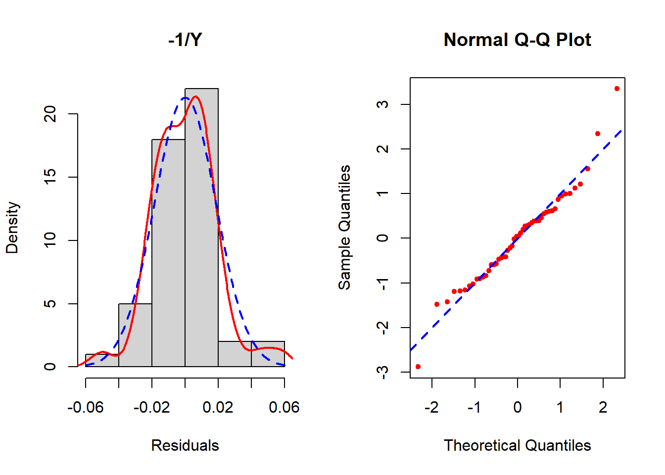
Figure 5.25: Checking the normality assumption (inverse outcome)
None seem to resolve the non-normality completely, but of these the inverse transformation is the best. See Section 5.19 for how to implement the Box-Cox transformation which potentially can improve upon these. In this example, Box-Cox turns out not to help much – after reading Section 5.19, come back and try it as an exercise to confirm that conclusion.