4.7 Confidence intervals and prediction intervals
When reporting a parameter estimate, also report a confidence interval for the parameter. A 95% confidence interval (CI) for a population parameter is a random interval that has 95% probability of containing the true parameter. For example, if (5.1%, 7.3%) is a 95% CI for the prevalence of some disease in a population, that means that there is a 95% chance that this interval contains the true prevalence.
We are going to look at three different kinds of intervals that you can create in simple linear regression: (1) CIs for regression coefficients, (2) a CI for the mean outcome, and (3) a prediction interval (PI) for an individual observation.
- The regression coefficients are the \(\beta\)s – the intercept and slope (for a continuous predictor) or the intercept and differences in mean outcome between levels and the reference level (for a categorical predictor).
- The estimated mean outcome is the value of the outcome on the regression line which we computed in Section 4.6.
- The predicted outcome for an individual observation is identical to the estimated mean outcome, but the PI for the outcome for an individual observation will be wider than the CI for the estimated mean outcome because individual observations are more variable than the mean.
4.7.1 CIs for regression coefficients
Earlier, we computed CIs for each of the individual regression coefficients using confint(fit).
##               2.5 %  97.5 %
## (Intercept) 2.72514 3.88305
## BMXWAIST    0.02208 0.03344
Based on this output, we conclude that a 95% CI for the population slope (\(\beta_1\)) of the regression of fasting glucose on waist circumference is 0.0221, 0.0334. Combining this with the regression coefficient and p-value from the earlier regression output, we would report this as follows: Waist circumference is significantly associated with fasting glucose (B = 0.0278; 95% CI = 0.0221, 0.0334; p <.001).
For a categorical predictor,
##                 2.5 % 97.5 %
## (Intercept)    5.8116 6.0730
## smokerPast     0.1864 0.6535
## smokerCurrent -0.0279 0.5380
Recall that the intercept (\(\beta_0\)) is the mean outcome at the reference level, and the other parameters are differences in mean between those levels and the reference level. Thus, a 95% CI for the population mean fasting glucose among never smokers is 5.8116, 6.0730. To get a CI for the mean at another level, re-level the predictor to make that level the reference level (see Section 4.4.3), re-fit the model, and re-compute the CI for the intercept.
A 95% CI for the population difference in mean fasting glucose between past and never smokers is 0.1864, 0.6535. We would report this as follows: Mean fasting glucose is significantly different between past and never smokers (B = 0.42; 95% CI = 0.19, 0.65; p <.001). To get a CI for a pairwise comparison between levels where neither is the reference level, re-level the predictor (see Section 4.4.3), re-fit the model, and re-compute the CI for the appropriate regression coefficient.
4.7.2 CI for the mean outcome
We already computed a CI for the mean outcome earlier when we used predict() along with interval = confidence. By way of reminder,
# Example 4.1 (continuous predictor)
predict(fit.ex4.1,
        newdata = data.frame(BMXWAIST = 100),
        interval = "confidence")
## fit lwr upr
## 1 6.08 5.984 6.177CIs for the mean over the entire range of \(X\) values are referred to as a confidence band since they visually form a band around the regression line. To visualize the confidence band for a continuous predictor, compute the CIs over the range of possible \(X\) values.
X <- seq(min(nhanesf$BMXWAIST, na.rm=T),
         max(nhanesf$BMXWAIST, na.rm=T), by = 1)
mypred.cont <- predict(fit.ex4.1,
                       newdata = data.frame(BMXWAIST=X),
                       interval="confidence")
This produces a matrix with one row for each \(X\) value and three columns – the estimated mean and the lower and upper confidence limits. View the \(X\) values along with the predictions by using data.frame to create a dataset with \(X\) and the values in mypred.cont.
##      X   fit   lwr   upr
## 1 63.2 5.059 4.826 5.291
## 2 64.2 5.086 4.859 5.314
## 3 65.2 5.114 4.892 5.336
## 4 66.2 5.142 4.925 5.359
## 5 67.2 5.170 4.957 5.382
## 6 68.2 5.197 4.990 5.405
In Figure 4.4, we plot fit vs. X to see the regression line (solid line), and each of lwr and upr vs. X to see the confidence band (dashed lines). With a reasonably large sample size, the confidence band will be quite narrow, so below it is plotted both on the original scale and zoomed in (using the ylim option to restrict the y-axis limits) to see the band more clearly.
par(mfrow=c(1,2))
plot(LBDGLUSI ~ BMXWAIST,   data = nhanesf,
     col="gray",
     ylab = "Fasting Glucose (mmol/L)",
     xlab = "Waist Circumference (cm)",
     las = 1, pch = 20, font.lab = 2, font.axis = 2, cex.axis = 0.75)
# NOTE: For lines() the arguments are x, y not y ~ x
lines(X, mypred.cont[, "fit"], col = "red",  lty = 1, lwd = 2)
lines(X, mypred.cont[, "upr"], col = "blue", lty = 5, lwd = 2)
lines(X, mypred.cont[, "lwr"], col = "blue", lty = 5, lwd = 2)

plot(LBDGLUSI ~ BMXWAIST,   data = nhanesf, ylim = c(4.5, 8.5),
     col="gray",
     ylab = "(zoomed in)",
     xlab = "Waist Circumference (cm)",
     las = 1, pch = 20, font.lab = 2, font.axis = 2, cex.axis = 0.75)
# NOTE: For lines() the arguments are x, y not y ~ x
lines(X, mypred.cont[, "fit"], col = "red",  lty = 1, lwd = 2)
lines(X, mypred.cont[, "upr"], col = "blue", lty = 5, lwd = 2)
lines(X, mypred.cont[, "lwr"], col = "blue", lty = 5, lwd = 2)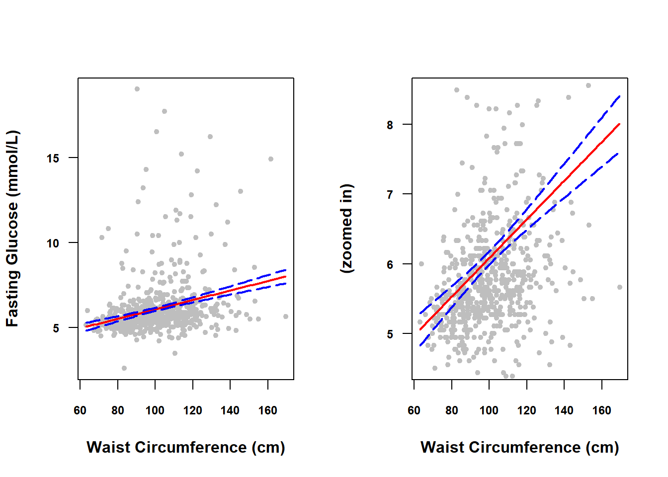
Figure 4.4: Confidence band for a continuous predictor
In general, the confidence band will be narrower in the middle of the predictor range and wider at the edges because we are more confident in the location of the middle of the line than we are about the location of the ends of the line. This could be shown mathematically but, just conceptually, consider that a slightly different sample of points would result in a slightly shifted and rotated line and that any rotation is going to have a greater impact on the ends of the line than the middle.
If the predictor is categorical, then rather than plotting over a continuous range of \(X\) values, we plot at the set of discrete levels of \(X\) (using levels()), as shown in Figure 4.5.
# Example 4.2 (categorical predictor)
X <- levels(nhanesf$smoker)
mypred.cat <- predict(fit.ex4.2,
                      newdata = data.frame(smoker=X),
                      interval="confidence")
data.frame(X, mypred.cat)
## X fit lwr upr
## 1 Never 5.942 5.812 6.073
## 2 Past 6.362 6.169 6.556
## 3 Current 6.197 5.946 6.448par(mfrow=c(1,2))
plot.default(nhanesf$LBDGLUSI ~ nhanesf$smoker,
col="gray",
ylab = "Fasting Glucose (mmol/L)",
xlab = "Smoking Status",
las = 1, pch = 20,
font.lab = 2, font.axis = 2, xaxt = "n")
axis(1, at = 1:3, labels = levels(nhanesf$smoker), font = 2)
# NOTE: For points() and lines() the arguments are x, y not y ~ x
points(1:3, mypred.cat[, "fit"], col = "red", pch = 20, cex = 1.5)
lines( 1:3, mypred.cat[, "fit"], col = "red")
lines( 1:3, mypred.cat[, "upr"], col = "blue", lty = 5, lwd = 2)
lines( 1:3, mypred.cat[, "lwr"], col = "blue", lty = 5, lwd = 2)
plot.default(nhanesf$LBDGLUSI ~ nhanesf$smoker, ylim = c(4.5, 8.5),
col="gray",
ylab = "(zoomed in)",
xlab = "Smoking Status",
las = 1, pch = 20,
font.lab = 2, font.axis = 2, xaxt = "n")
axis(1, at = 1:3, labels = levels(nhanesf$smoker), font = 2)
# NOTE: For points() and lines() the arguments are x, y not y ~ x
points(1:3, mypred.cat[, "fit"], col = "red", pch = 20, cex = 1.5)
lines( 1:3, mypred.cat[, "fit"], col = "red")
lines( 1:3, mypred.cat[, "upr"], col = "blue", lty = 5, lwd = 2)
lines( 1:3, mypred.cat[, "lwr"], col = "blue", lty = 5, lwd = 2)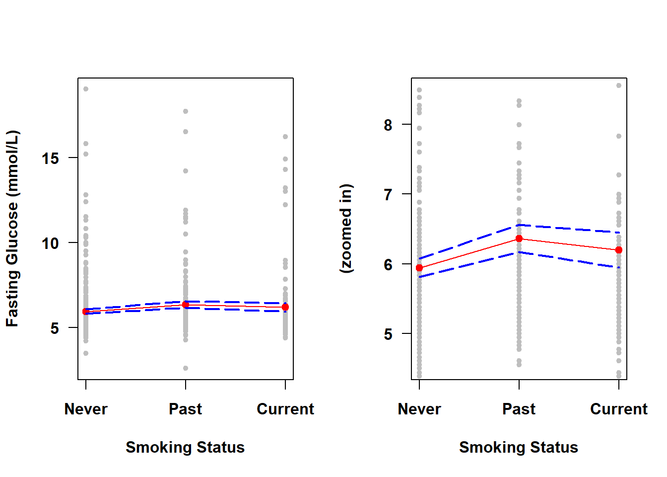
Figure 4.5: Confidence band for a categorical predictor
Unlike for a continuous predictor, the width of the confidence band is not necessarily greater on the “ends” when you have a categorical predictor. The width of the band now is instead related only to the sample size at each level of \(X\) – this dataset contains more never smokers so the CI for the prediction is narrower at that level.
4.7.3 PI for an individual observation
The third type of interval of interest is a prediction interval (PI) for the outcome for an individual observation at a specific predictor value. It turns out that the estimated value of the mean outcome and the predicted value for an individual’s outcome are identical, but their intervals are not. The PI for an individual’s outcome will be wider than the CI for the mean outcome – individuals are more variable than the average of individuals.
A 95% prediction interval for the outcome \(Y\) for an individual with a specific predictor value \(X=x\) is interpreted as follows: Among all individuals in the population with \(X=x\), we expect 95% of them to have outcome values within the 95% prediction interval.
In predict(), add interval = "prediction" to compute the PI for an individual observation.
# Example 4.1 (continuous predictor)
predict(fit.ex4.1,
        newdata = data.frame(BMXWAIST = 100),
        interval = "prediction")
## fit lwr upr
## 1 6.08 3.089 9.071The estimated average fasting glucose for individuals in the population with a waist circumference of 100 cm is 6.08 mmol/L, and we expect 95% of such individuals to have fasting glucose between 3.09 and 9.07 mmol/L.
# Example 4.2 (categorical predictor)
predict(fit.ex4.2,
        newdata = data.frame(smoker = "Current"),
        interval = "prediction")
## fit lwr upr
## 1 6.197 3.043 9.352The average fasting glucose for individuals who are current smokers is 6.20 mmol/L, and we expect 95% of current smokers to have a fasting glucose between 3.04 and 9.35 mmol/L.
The PIs for individual observations over a range of \(X\) values form a prediction band. To visualize the prediction band, use the same code as in Section 4.7.2 but with interval="prediction" instead of interval="confidence" in the call to predict(). The results for Examples 4.1 and 4.2 are shown in Figure 4.6 and Figure 4.7, respectively.
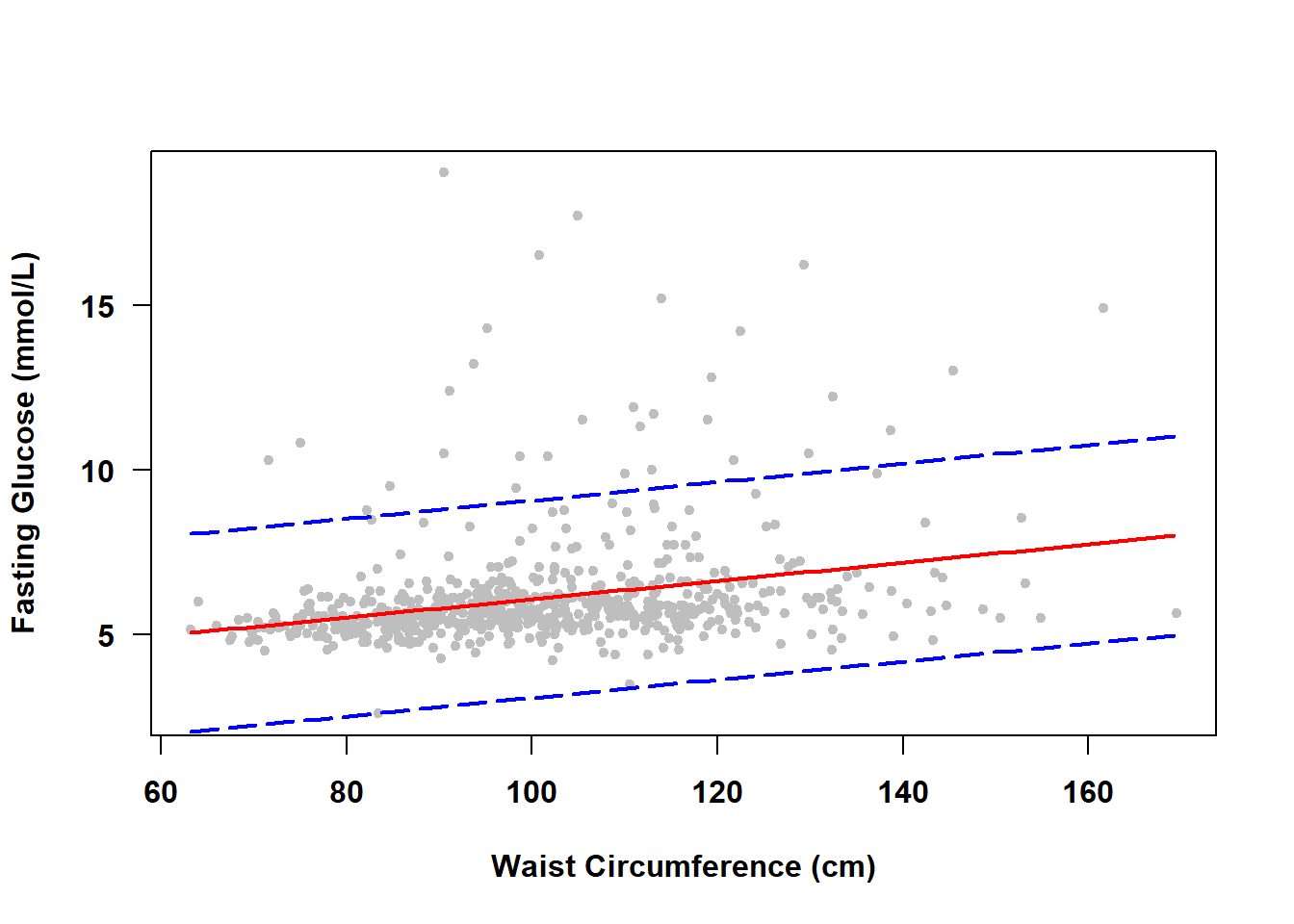
Figure 4.6: Prediction band for a continuous predictor
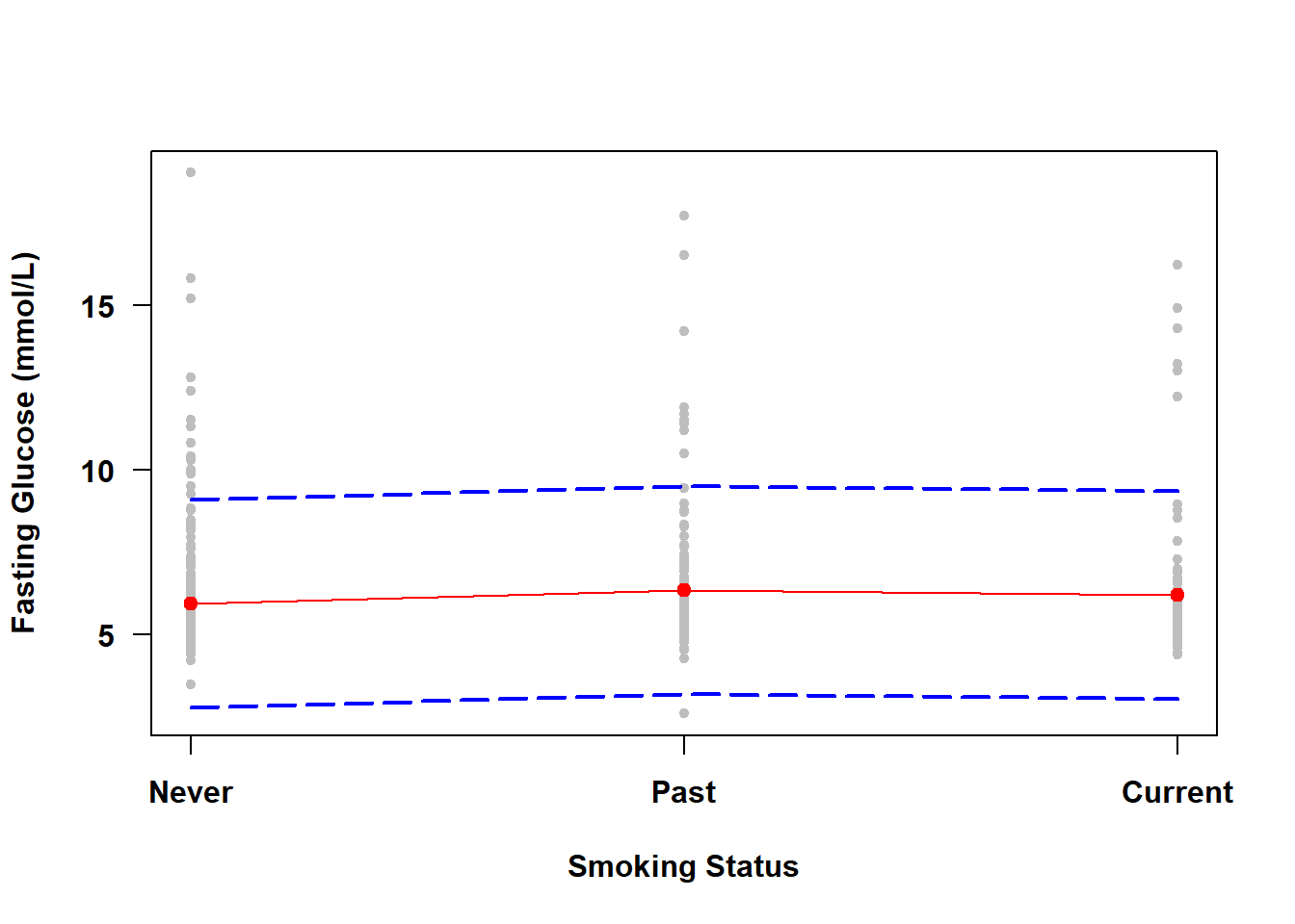
Figure 4.7: Prediction band for a categorical predictor
There is no need to zoom in this time because the prediction band is quite wide. Since we are less confident in the outcome for an individual observation than for the mean of individual observations, a prediction band will always be wider than a confidence band.
NOTE: As the sample size increases, a prediction band will become more accurate but will always be wide since it captures 95% of the observations. A confidence band, however, will get narrower as the sample size increases.
In summary, you can obtain three kinds of intervals from a regression – for the population regression coefficients, for the population mean outcome, and for the outcome for an individual observation. For the mean and individual the centers of the intervals are the same, but the PI for an individual observation will always be wider than the CI for the mean.