8.7 Weighted survival analysis
To incorporate a complex survey design into a survival analysis, use
svykm()to compute a weighted Kaplan-Meier estimate of the survival function,svylogrank()to carry out a weighted log-rank test to compare survival curves between groups, andsvycoxph()to carry out weighted Cox regression.
8.7.1 Weighted Kaplan-Meier estimate of the survival function
Example 8.4: Using the NHANES 2017-2018 data (nhanes1718_rmph.Rdata), estimate the weighted Kaplan-Meier estimate of the survival function for time to first diagnosis of asthma. The time variable is age when first had asthma (MCQ025) and the event indicator is “Ever been told you have asthma” (MCQ010).
We need an event indicator that is 1 for those who have been told they have asthma and 0 otherwise, and a time variable that is the age when told one first had asthma for those who have been told and current age otherwise (censored asthma age). Format the event indicator variable and then fill in current age for those without asthma.
NOTE: This step is needed for the Kaplan-Meier estimator, log-rank test, and Cox regression.
## [1] "Yes" "No"nhanes.mod$asthma <- as.numeric(nhanes.mod$MCQ010 == "Yes")
table(nhanes.mod$MCQ010, nhanes.mod$asthma, useNA = "ifany")##
## 0 1 <NA>
## Yes 0 1325 0
## No 7563 0 0
## <NA> 0 0 366# Create a copy of the age variable
nhanes.mod$asthma_age <- nhanes.mod$MCQ025
# For those with asthma = 0, set asthma age to current age
SUB <- complete.cases(nhanes.mod$asthma) & nhanes.mod$asthma == 0
nhanes.mod$asthma_age[SUB] <- nhanes.mod$RIDAGEYR[SUB]# Check derivation
# For !SUB, the difference between these should be 0 or NA
# (asthma_age is MCQ025)
summary(nhanes.mod$MCQ025[ !SUB] -
nhanes.mod$asthma_age[!SUB])
# For SUB, this should be all missing
summary(nhanes.mod$MCQ025[SUB])
# For !SUB, the difference between these should be 0
# (asthma_age is RIDAGEYR)
summary(nhanes.mod$RIDAGEYR[ SUB] -
nhanes.mod$asthma_age[SUB])
# (results not shown)Next, re-create the design object so that these new variables are available for weighted analyses. The asthma variables were part of the NHANES interview, and no other variables are included in this analysis, so use the interview design weights.
library(survey)
options(survey.lonely.psu = "adjust")
options(survey.adjust.domain.lonely = TRUE)

design.INT <- svydesign(strata=~SDMVSTRA, id=~SDMVPSU, weights=~WTINT2YR,
                        nest=TRUE, data=nhanes.mod)
Use svykm() and plot() to estimate and plot the survival function (Figure 8.6).
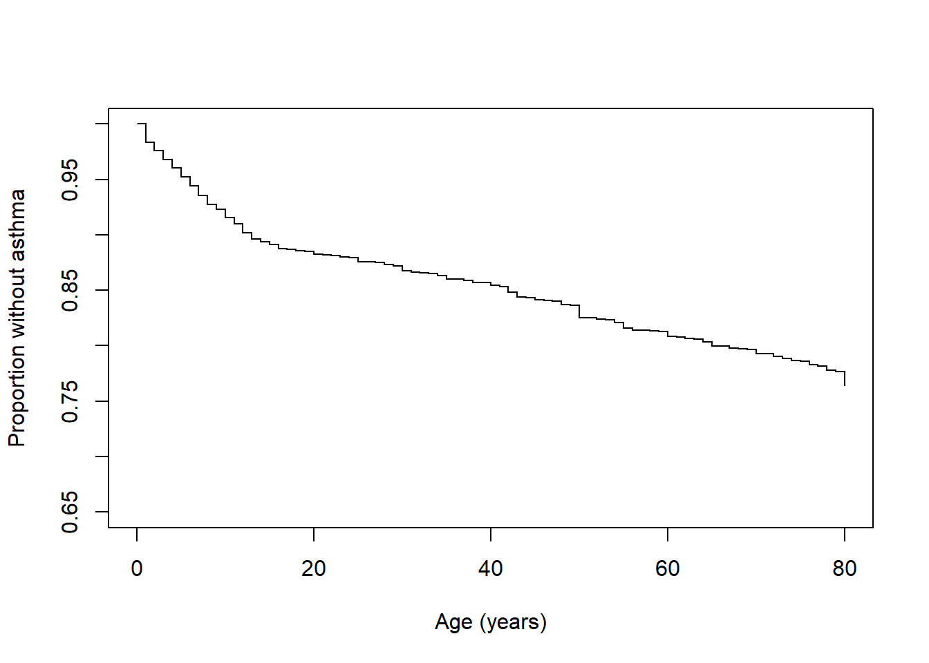
Figure 8.6: Weighted Kaplan-Meier survival function
Conclusion: We see that the proportion without asthma drops rapidly before age 20 years, indicating the greatest risk of an asthma diagnosis is in childhood. However, as the survival curve continues to decrease over the lifespan, adults who have not yet been diagnosed with asthma are still at risk.
8.7.2 Weighted log-rank test for comparing groups
To compare groups, use svykm with a factor variable on the right-hand side of the formula, and then svylogrank to carry out the log-rank test.
NOTE: If you have not already done so, format the event indicator and time variable (see Section 8.7.1).
Example 8.4 (continued): Using the NHANES 2017-2018 data (nhanes1718_rmph.Rdata), use a weighted log-rank test to compare time to first diagnosis of asthma between race/ethnicity groups. The race/ethnicity variable was also in the interview, so we can continue using the design object that includes the interview weights.
Figure 8.7 illustrates the comparison of weighted survival functions between race/ethnicity groups.
# When plotting svykm objects, the lty option must be in a list.
# When including lty, ylim must also be in a list
# (without lty, ylim works without being in a list)
plot(km.ex8.4b,
     xlab = "Age (years)",
     ylab = "Proportion without asthma",
     pars = list(lty=1:4), ylim = list(c(0.65, 1)))
legend(45, 1, levels(nhanes.mod$race_eth)[c(2,4,1,3)],
       lty = (1:4)[c(2,4,1,3)])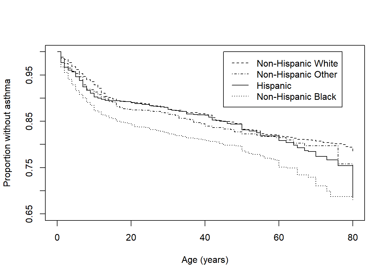
Figure 8.7: Weighted Kaplan-Meier survival function by race/ethnicity
# WARNING: svylogrank() will fail if there are missing values.
# Create a domain with only complete cases
nhanes.mod <- nhanes.mod %>%
  mutate(domain_asthma = complete.cases(asthma_age) & complete.cases(asthma) &
                         complete.cases(race_eth))

# Re-create the design to include the new domain variable
design.INT <- svydesign(strata=~SDMVSTRA, id=~SDMVPSU, weights=~WTINT2YR,
                        nest=TRUE, data=nhanes.mod)

# Subset the design to do a domain analysis
design_asthma <- subset(design.INT, domain_asthma)

# Log-rank test
svylogrank(Surv(asthma_age, asthma) ~ race_eth, design = design_asthma)[[2]]
## Chisq p
## 29.330856009 0.000001908Conclusion: Time to first diagnosis of asthma differs significantly between race/ethnicity groups (p < .001). As shown in Figure 8.7, non-Hispanic Black individuals have the greatest proportion of individuals with asthma at any given age, starting from childhood and persisting across the lifespan.
8.7.3 Weighted Cox regression
8.7.3.1 Fitting the model
Use svycoxph() to fit a weighted Cox proportional hazards regression. The current functions do not have an option to change the DF from the default. An exception is the function svycontrast_design_df() (in Functions_rmph.R) which uses the design DF by default, with an option to use the residual DF.
NOTE: If you have not already done so, format the event indicator and time variable (see Section 8.7.1).
Example 8.5: Using the NHANES 2017-2018 data (nhanes1718_rmph.Rdata), compare time to first diagnosis of asthma between race/ethnicity groups, adjusted for gender (RIAGENDR), using a Cox proportional hazards regression.
The results are shown in Table 8.7.
car::Anova(cox.ex8.5, type = 3)
summary(cox.ex8.5)
cbind("AHR" = exp(summary(cox.ex8.5)$coef[, "coef"]),
              exp(confint(cox.ex8.5)),
      "p"   = summary(cox.ex8.5)$coef[, "Pr(>|z|)"])
# (results not shown)library(gtsummary)
# Table of regression coefficients
t1 <- cox.ex8.5 %>%
tbl_regression(estimate_fun = function(x) style_number(x, digits = 3),
label = list(race_eth ~ "Race/Ethnicity",
RIAGENDR ~ "Gender")) %>%
modify_column_hide(p.value) %>%
modify_caption("Weighted Cox regression results for time to asthma
vs. race/ethnicity, adjusted for gender")## Stratified 1 - level Cluster Sampling design (with replacement)
## With (30) clusters.
## svydesign(strata = ~SDMVSTRA, id = ~SDMVPSU, weights = ~WTINT2YR,
## nest = TRUE, data = nhanes.mod)# Table of hazard ratios
t2 <- cox.ex8.5 %>%
tbl_regression(exponentiate = T, # HR = exp(B)
estimate_fun = function(x) style_number(x, digits = 3),
pvalue_fun = function(x) style_pvalue(x, digits = 3),
label = list(race_eth ~ "Race/Ethnicity",
RIAGENDR ~ "Gender")) %>%
add_global_p(keep = T)## Stratified 1 - level Cluster Sampling design (with replacement)
## With (30) clusters.
## svydesign(strata = ~SDMVSTRA, id = ~SDMVPSU, weights = ~WTINT2YR,
## nest = TRUE, data = nhanes.mod)TABLE <- tbl_merge(
tbls = list(t1, t2),
tab_spanner = c("**Regression Coefficient**", "**Adjusted Hazard Ratio**")
) %>%
modify_footnote(everything() ~ NA, abbreviation = TRUE) %>%
modify_header(update = list(
estimate_1 = "**log(AHR)**",
estimate_2 = "**AHR**"
))| Characteristic |
Regression Coefficient
|
Adjusted Hazard Ratio
|
|||
|---|---|---|---|---|---|
| log(AHR) | 95% CI | AHR | 95% CI | p-value | |
| Race/Ethnicity | <0.001 | ||||
| Hispanic | — | — | — | — | |
| Non-Hispanic White | -0.083 | -0.316, 0.151 | 0.921 | 0.729, 1.162 | 0.487 |
| Non-Hispanic Black | 0.314 | 0.071, 0.557 | 1.369 | 1.074, 1.745 | 0.011 |
| Non-Hispanic Other | 0.028 | -0.391, 0.446 | 1.028 | 0.677, 1.562 | 0.897 |
| Gender | 0.117 | ||||
| Male | — | — | — | — | |
| Female | 0.138 | -0.035, 0.310 | 1.148 | 0.966, 1.364 | 0.117 |
| Abbreviations: CI = Confidence Interval, HR = Hazard Ratio, NA | |||||
Conclusion: After adjusting for gender, time to first diagnosis of asthma is significantly different between race/ethnicity groups (p < .001). Non-Hispanic Black participants have 36.9% greater hazard of asthma diagnosis than Hispanic participants. Note that the AHR for non-Hispanic White participants is < 1, so the disparity between non-Hispanic Black and non-Hispanic White is even greater than 36.9%. To estimate it, divide the two AHRs, 1.369/0.921 = 1.486 to see that non-Hispanic Black participants have 48.6% greater hazard of an asthma diagnosis than non-Hispanic White participants. If you also want a 95% confidence interval and a p-value to go along with this estimate, then re-level the race/ethnicity variable to make non-Hispanic White the reference level, refit the model, and then examine the effect for non-Hispanic Black, which would then be a comparison with non-Hispanic White.
8.7.3.2 Exclude cases with zero weights
Unlike the other functions we have used in this chapter, svycoxph() returns an error if there are any cases with 0 weight. To avoid this, use a domain analysis to exclude these cases. If you were already using a domain analysis, modify that domain to also exclude these cases. For example, in the NHANES dataset, there are some cases with exam weights of 0 (those not in the examination subsample).
8.7.3.3 Interactions
Including an interaction in the model and estimating effects for one variable at levels of another proceeds as described for weighted binary logistic regression above.
Example 8.5 (continued): Does the effect of body mass index (BMXBMI) on time to asthma differ between race/ethnicity groups, adjusted for gender? Estimate the BMI effect at each level of race/ethnicity.
Since BMI was only collected in the examination subsample, we must use the examination weights when specifying the sample design (and use a domain analysis that excludes those with zero weights; see Section 8.7.3.2).
cox.ex8.5.int <- svycoxph(Surv(asthma_age, asthma) ~ race_eth + RIAGENDR +
                            BMXBMI + race_eth:BMXBMI,
                          design = design.MEC.pos.weights)
car::Anova(cox.ex8.5.int, type = 3)
## Analysis of Deviance Table (Type III tests)
##
## Response: Surv(asthma_age, asthma)
## Df Chisq Pr(>Chisq)
## race_eth 3 6.73 0.081 .
## RIAGENDR 1 3.55 0.060 .
## BMXBMI 1 1.53 0.216
## race_eth:BMXBMI 3 5.09 0.165
## ---
## Signif. codes: 0 '***' 0.001 '**' 0.01 '*' 0.05 '.' 0.1 ' ' 1rbind(
"BMI @ Hispanic" = svycontrast_design_df(cox.ex8.5.int,
c("BMXBMI" = 1),
EXP=T),
"BMI @ NH White" = svycontrast_design_df(cox.ex8.5.int,
c("BMXBMI" = 1,
"race_ethNon-Hispanic White:BMXBMI" = 1),
EXP=T),
"BMI @ NH Black" = svycontrast_design_df(cox.ex8.5.int,
c("BMXBMI" = 1,
"race_ethNon-Hispanic Black:BMXBMI" = 1),
EXP=T),
"BMI @ NH Other" = svycontrast_design_df(cox.ex8.5.int,
c("BMXBMI" = 1,
"race_ethNon-Hispanic Other:BMXBMI" = 1),
EXP=T)
)## est lower upper
## BMI @ Hispanic 0.9823 0.9525 1.013
## BMI @ NH White 1.0047 0.9808 1.029
## BMI @ NH Black 0.9945 0.9785 1.011
## BMI @ NH Other 1.0211 0.9962 1.047Conclusion: After adjusting for gender, the effect of body mass index on time to asthma does not significantly differ between race/ethnicity groups (p = .165).