6.13 Outliers
Outliers are observations with predictions that are very far from their observed values. In linear regression, outliers signaled a possible problem with the normality and/or constant variance assumptions, particularly in small samples. Logistic regression does not have these assumptions; however, it is still useful to examine outliers to find observations that are not predicted well by the model.
In a logistic regression, the observed values are always each 0 or 1 (even if the response is coded as a factor, numerically glm() uses 0s and 1s) and the predicted probabilities are always between 0 and 1, so the differences between these are always between –1 and 1. The residuals in a logistic regression, called deviance residuals, are more complex, however, than simple differences between observed outcomes and predicted probabilities. For a glm object, the usual residual functions resid(), rstandard(), and rstudent() compute deviance residuals and their standardized and Studentized counterparts, respectively.
Examine outliers by highlighting points on a residual plot and examining their predictor and outcome values. Again, here we are simply examining observations that are fit poorly by the model. After identifying them, we do not remove them from the model, although you could do a sensitivity analysis to evaluate their impact on your conclusions.
Example 6.3 (continued): Look for outliers in the model that does not include an interaction. The cutoff you choose here is arbitrary. In this example, a cutoff of 2.5 highlighted a few observations and you can see from Figure 6.6 that the two with the most negative residuals especially seem to stand out as being highly unusual.
## [1] 4car::residualPlots(fit.ex6.3.adj, terms = ~ 1,
tests = F, quadratic = F, fitted = T,
type = "rstudent", pch = 20, col = "gray")
# NOTE: For points() the arguments are x, y not y ~ x
points(logit(fitted(fit.ex6.3.adj))[SUB],
RSTUDENT[SUB],
pch=20, cex=1.5)
abline(h = c(-2.5, 2.5), lty = 2)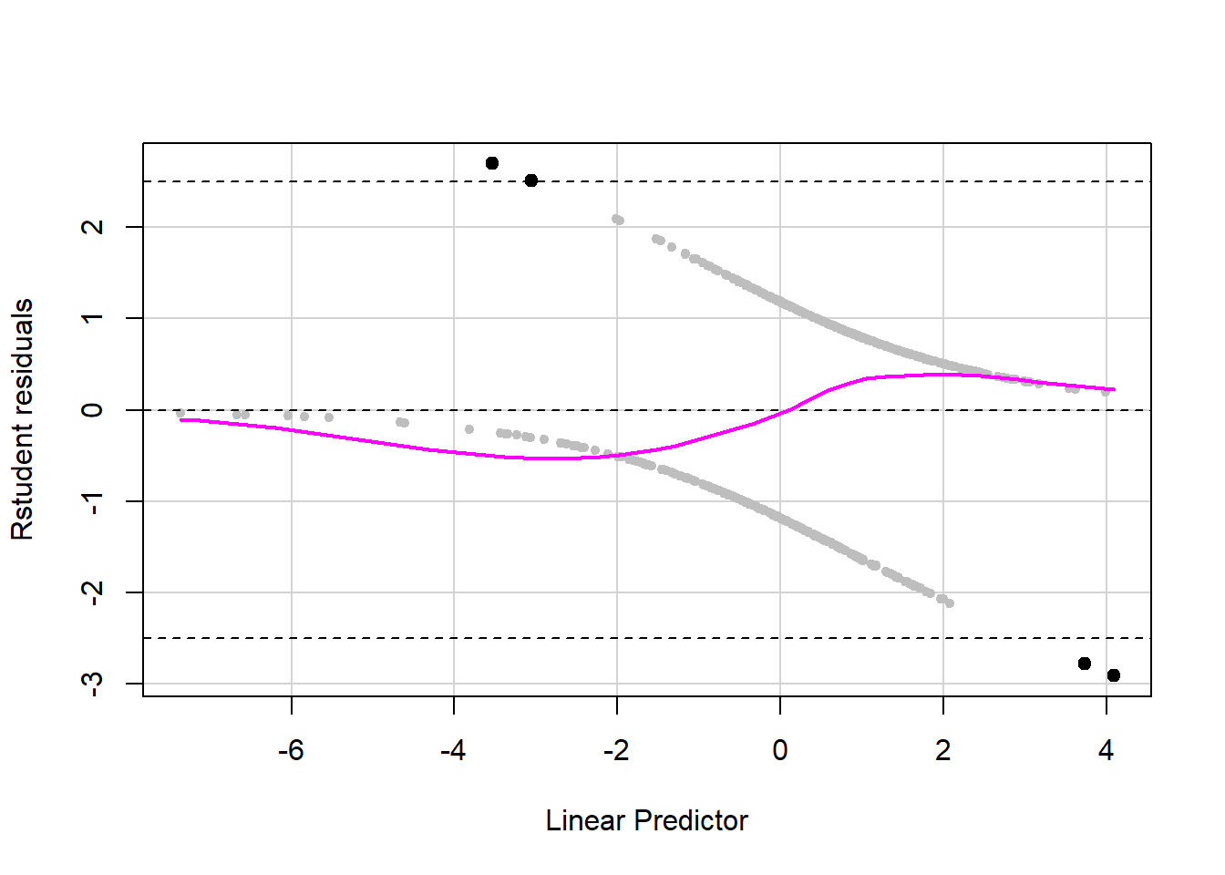
Figure 6.6: Identifying outliers in a logistic regression
Outliers in a logistic regression are observations with either (a) \(Y = 1\) but predictors at levels at which the predicted probability is very low (resulting in a large positive residual) or (b) \(Y = 0\) but predictors at levels at which the predicted probability is very high (resulting in a large negative residual). By way of reminder, here are the AORs for the terms in this model.
##                                 AOR 2.5 % 97.5 %
## alc_agefirst                  0.759 0.718  0.800
## demog_age_cat626-34           0.744 0.387  1.409
## demog_age_cat635-49           0.447 0.247  0.791
## demog_age_cat650-64           0.502 0.275  0.891
## demog_age_cat665+             0.279 0.152  0.502
## demog_sexMale                 0.941 0.684  1.291
## demog_income$20,000 - $49,999 0.588 0.347  0.987
## demog_income$50,000 - $74,999 0.924 0.507  1.680
## demog_income$75,000 or more   0.697 0.421  1.139
If we examine the observation with the largest negative residual more closely, we see that it falls into the latter category. This individual did not use marijuana (\(Y = 0\)) but is in the income group with the highest odds of lifetime marijuana use and has an extremely young age of first alcohol use, also corresponding to greater odds of the outcome, and these discrepancies result in a large negative residual. If one had access to the raw data, it would be worth checking to see if the value of 3 for alc_agefirst is a data entry error.
##  10412   3043  48455  40288
##  2.510  2.695 -2.909 -2.776
# Examine that row
nsduh[c("48455"),
c("mj_lifetime",
"alc_agefirst",
"demog_age_cat6",
"demog_sex",
"demog_income")]## mj_lifetime alc_agefirst demog_age_cat6 demog_sex demog_income
## 48455 No 3 65+ Male Less than $20,000