5.7 Residuals
Many regression concepts and diagnostic tools we will discuss use residuals to diagnose assumptions about the error term \(\epsilon\) – the part of the outcome not explained by the MLR model. Based on the MRL model
\[Y = \beta_0 + \beta_1 X_1 + \beta_2 X_2 + \ldots + \beta_K X_K + \epsilon\]
we get the following formula for the predicted value for the \(i^{th}\) observation given its predictor values:
\[\hat{y_i} = \hat\beta_0 + \hat\beta_1 x_{i1} + \hat\beta_2 x_{i2} + \ldots + \hat\beta_K x_{iK}.\]
The hat (\(\hat{ }\)) on top of a term signifies that it is a prediction (of \(y_i\)) or estimate (of one of the \(\beta\)s), and the lowercase \(x\)’s are the specific values of the predictors at which we are computing the predicted value. \(\hat{y_i}\) is our best guess of the outcome given these predictor values. Notice that there is no random error term in this second equation – this is not the equation of a model but rather the equation for obtaining a prediction and, given the fitted model and a set of predictor values, the prediction is the same every time.
Every individual with the same set of predictor values has the same predicted value of the outcome. But, of course, not every individual has the same observed value of the outcome. For each individual, the difference between their observed and predicted outcome is their residual. If an observation has a residual of 0, then the prediction from the model is exactly the same as the observed value – the model captures this observation perfectly. If an observation has a large residual, however, then the prediction from the model is far from the observed value – the model does not capture this observation well.
The prediction for the \(i^{th}\) observation, \(\hat{y_i}\), is also called the fitted value. The unstandardized residual is the difference between the observed outcome and the fitted value. For example, if \(\hat\beta_0\) and \(\hat\beta_1\) are the estimates of the intercept \(\beta_0\) and slope \(\beta_1\) in a SLR with a continuous predictor, then the residual \(e_i\) for the \(i^{th}\) observation is expressed as
\[e_i = y_i - \hat{y_i} = y_i - \left(\hat\beta_0 + \hat\beta_1 x_i\right).\]
Visually, a residual is the perpendicular distance from an observed value to the regression line, as shown in Figure 5.4 for two observations. Points above the line have positive residuals, and those below the line have negative residuals.
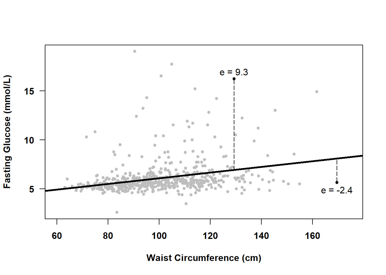
Figure 5.4: What is a residual?
5.7.1 Computing residuals
Many diagnostic tools that use residuals automatically compute them for you, but there may be times you need to compute them yourself. The basic definition of a residual given in Section 5.7 is for an unstandardized residual – the raw difference between the observed and fitted values. Unstandardized residuals are appropriate if you want to examine the residuals on the same scale as the outcome. However, if you want to compare the magnitude of residuals to an objective standard, then you must first convert them to a standardized scale.
Standardized residuals are residuals divided by an estimate of their standard deviation, the result being that they have a standard deviation very close to 1, no matter what the scale of the outcome. Studentized residuals are similar to standardized residuals except that, for each case, the residual is divided by the standard deviation estimated from the regression with that case removed. For Studentized residuals, the objective standard to which they may be compared is the \(t\) distribution with degrees of freedom equal to the model residual degrees of freedom minus 1. For large sample sizes, this is very close to a standard normal distribution and Studentized residuals can be thought of as the number of standard deviations a case’s outcome value is away from the regression line. For example, a Studentized residual of 2 corresponds to a point that is approximately 2 standard deviations above the regression line.
The residuals() (or resid()), rstandard(), and rstudent() functions compute unstandardized, standardized, and Studentized residuals, respectively. For example,
r1  <- resid(fit.ex5.1)
r2  <- rstandard(fit.ex5.1)
r3  <- rstudent(fit.ex5.1)
# Compare means and standard deviations
COMPARE <- round(data.frame(Mean = c(mean(r1), mean(r2), mean(r3)),
                            SD   = c(sd(r1),   sd(r2),   sd(r3))), 5)
rownames(COMPARE) <- c("Unstandardized", "Standardized", "Studentized")
COMPARE
## Mean SD
## Unstandardized 0.00000 1.501
## Standardized 0.00004 1.002
## Studentized 0.00234 1.016You can also extract the unstandardized residuals from an lm() object.
All three types of residuals have a mean of approximately 0 (for unstandardized residuals, it will be exactly 0), and standardized and Studentized residuals each have a standard deviation that is approximately 1. This makes standardized and Studentized residuals each comparable to an objective standard. As shown in Figure 5.5, the distribution of all three types of residuals will have approximately the same shape.
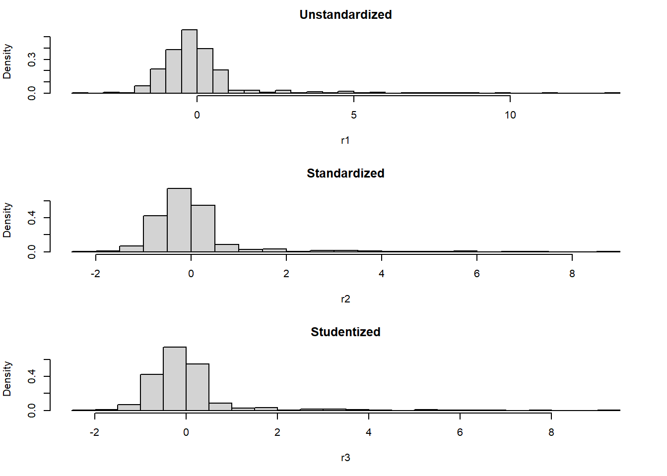
Figure 5.5: Three different types of residuals